
Microsoft Excel, Microsoft Word, and Microsoft Outlook are the heavyweights in the Microsoft Office suite. It is no secret that Microsoft Office, especially Excel, is a boon to all entrepreneurs and data entry professionals whose sole job is to keep data and information organised online. It is a standard spreadsheet tool that is needed in most industries these days.
Excel 2016 is a suite of tools that enable a user to analyse, organise, manipulate, and format data in a spreadsheet. It is the lifeblood of all corporate houses, financial outfits, and research firms, but its needs are not just limited to those users. People have started using Excel in their daily lives too, whether it is for managing a household budget, recording their students’ attendance, or maintaining an inventory.
Excel 2016 is full of tips and tricks that will surprise you and make your life easier. Let’s check out the top 11 Excel 2016 tips and tricks that you should know!
Microsoft Excel: Tips & Tricks
1. Add or Remove Cells, Rows or Columns
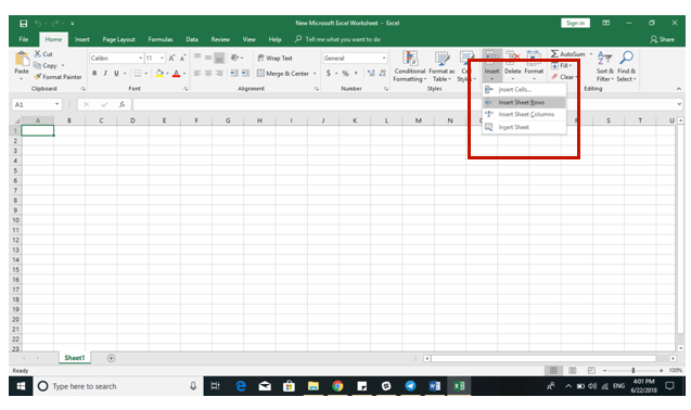
Inserting or deleting cells, rows or columns in an Excel is easy with the commands “Insert Cells” and “Delete Cells.” You have to click the Insert button and select the option you want.
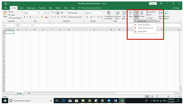
Similarly, you can use the Delete option and choose the appropriate icon to delete a cell, row or column.
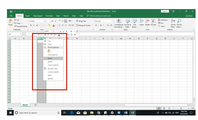
To make things easier, you can also right-click on any row or column to add/delete a cell.
2. Resize Rows and Columns
The size of Excel’s rows and columns is pretty standard, so there’s a fair chance that you will have to adjust their size to accommodate all the data that you need to put in there.
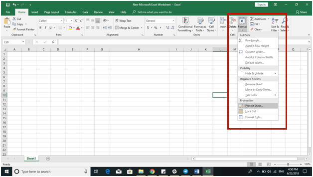
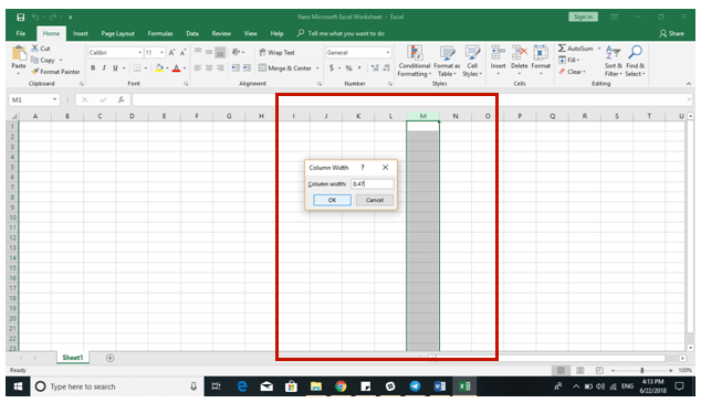
It is relatively simple to change the width or height of a cell by going to the Home icon, clicking Format, and choosing Column Width.
Then you need to enter the number you’d like the cell to be set to and click OK.
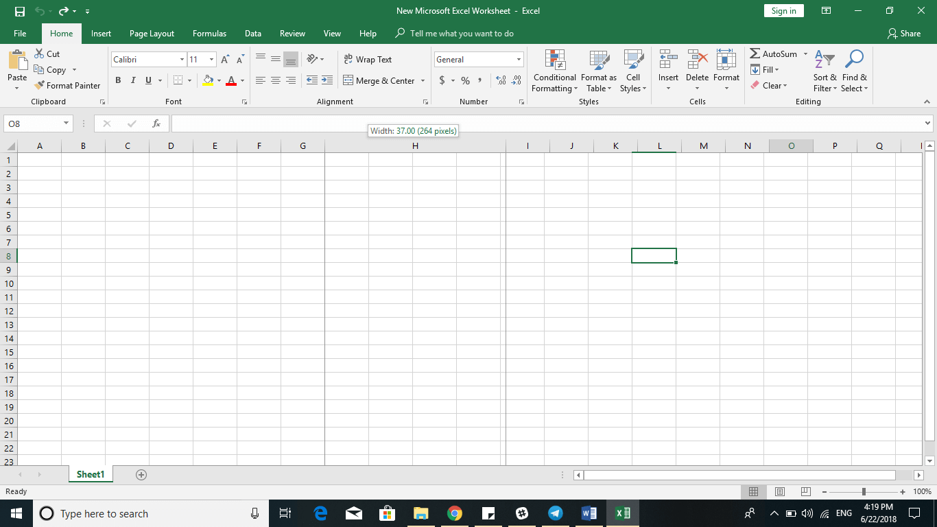
It is also straightforward to manually adjust the rows and columns by placing the pointer anywhere between a row and a column and dragging and expanding the row/column till you reach your desired size.
3. Freeze Panes
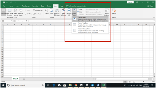
The Freeze Panes function comes in quite handy when you want to scroll through a section of the spreadsheet without losing focus on a specific part of the sheet.
To Freeze Panes, select the column or row where the data begins, select the View option, and click the menu that says Freeze Panes to do the job!
4. Change the Alignment of Text in the Cells
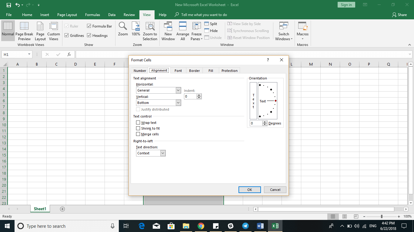
It is easy to use the Format Cells dialogue in Excel to create labels or a register and adjust text alignment in a cell. To apply the formatting, right-click on the selected row/column and hit Format Cells.
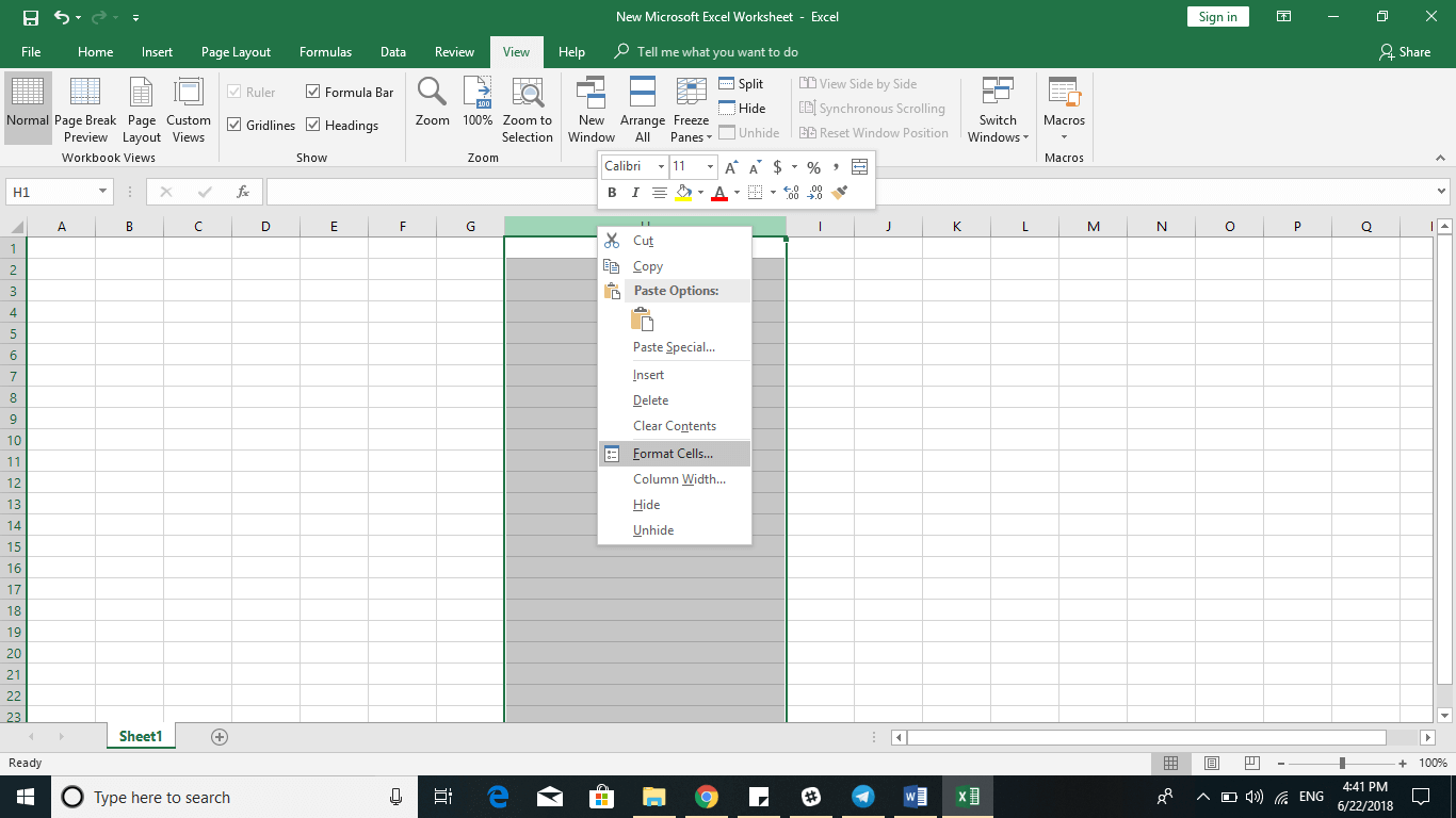
Then choose the Alignment tab, change the text orientation as needed, and click OK.
5. Cell Prevention to Prevent Someone from Editing a Particular Part of the Sheet
The Cell Prevention feature can prove to be quite beneficial if you wish to prevent someone from editing a specific part of the Excel. It dramatically reduces accidental edits and saves you a lot of extra work.
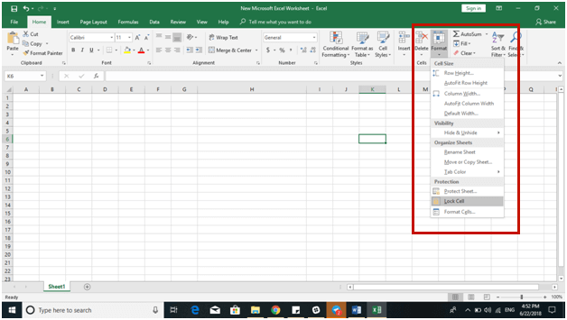
Protecting a group of cells is easy. Just turn on the Protect Sheet feature in the Format menu.
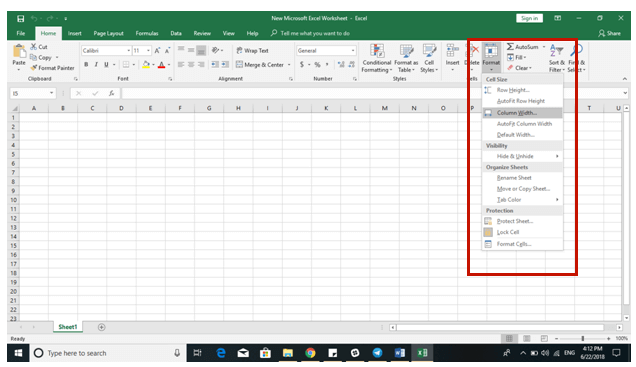
Choose all the desired options, including the password to protect the sheet, and click ok.
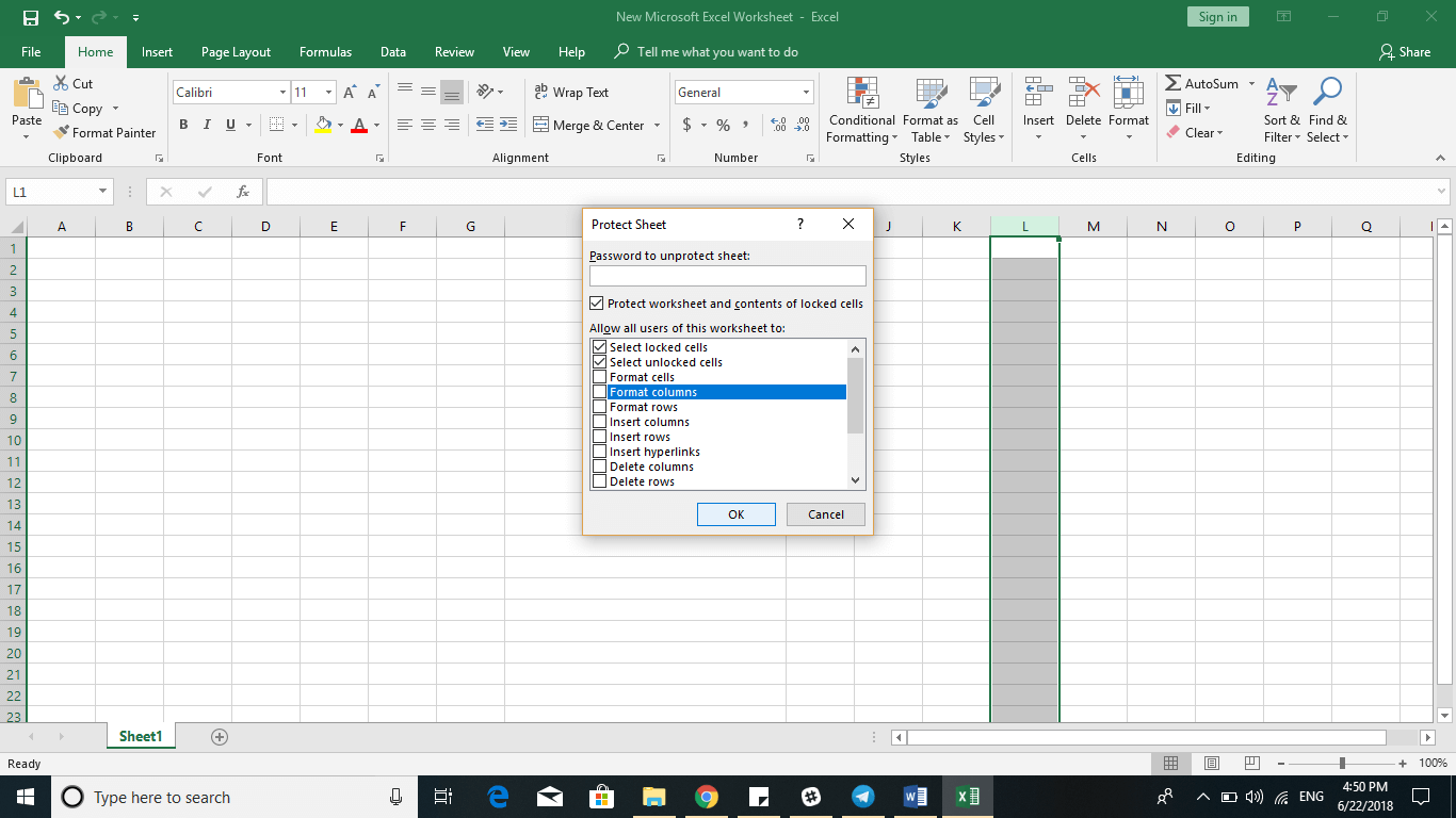
You can also lock a cell if you wish to prevent someone from editing a bunch of rows or columns. To do this, select the row and columns that you want to keep pristine and hit Format → Lock Cell. And that is it.
6. Apply Special Formatting in Cells to Currencies and Numbers
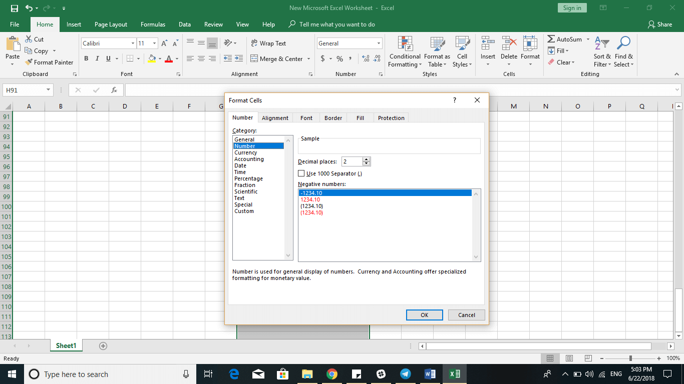
If you wish to insert a decimal or a particular currency in any of the cells, rows or columns, you can do that in a jiffy.
Go to Format Cells by right-clicking on the selected column/row and clicking on Numbers to make the desired changes to the numbers or the currency of a cell.
7. Sum, Average, Count, Max, Min – 5 Functions You Cannot Do Without in Excel
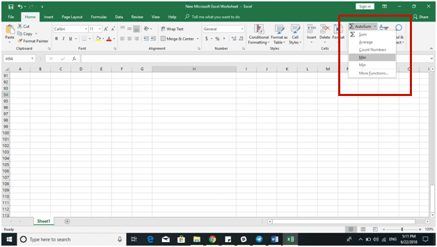
The one real power of Excel undoubtedly lies in its formulas and functions. If you do not know how to apply formulas in Excel, you know maybe 40% of the functions of Excel. Hence, it is pertinent to identify the five essential functions in Excel: Sum, Count, Average, Max, and Min. Let’s check out what these functions do and how to apply them!
- Sum – Calculates the total sum of the selected cells
- Count – Counts the number of values in the selected cells, leaving empty cells or those that have no numeric data
- Average – Calculates the average of the selected cells
- Min – Demonstrates the minimum value of the selected cells
- Max – Demonstrates the maximum value of the selected cells
To use a function, go to Home, click on AutoSum, go to the drop-down menu and use the appropriate function you wish to apply to a group of cells. Before doing that, do not forget to select the group of cells where you want to apply the function.
8. Manipulate and Create Charts
Creating and manipulating charts is probably the hallmark feature of Excel. It enables users to present their data in a visually well-formed manner. Excel significantly helps ease the process.
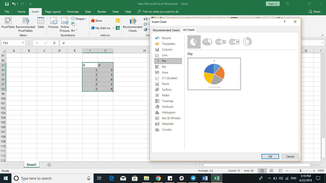
To do this, highlight the part of the spreadsheet you wish to manipulate, click on the Insert tab and then choose the All Charts option from the Recommended Charts icon.
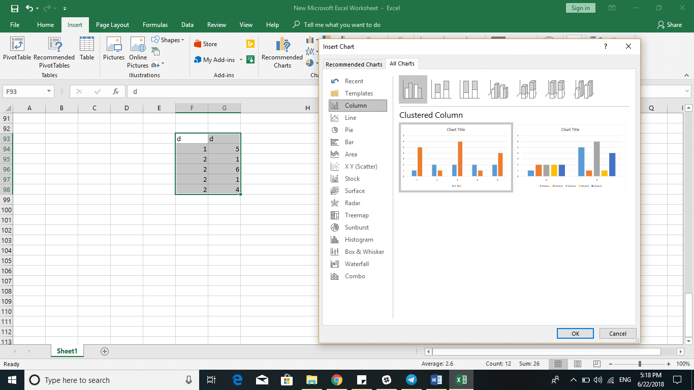
You can even see a preview by hovering over a sample to see the chart’s final result. Once you are satisfied, click ok to insert the chosen chart into the spreadsheet.
9. Reveal Formulas
Revealing all your formulas is probably the best way to validate all the calculations in your workbook. For example, the data shown below:

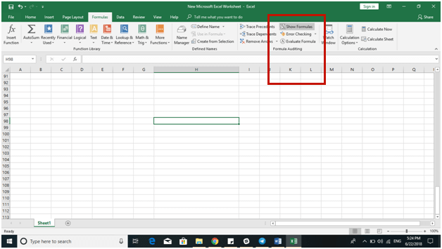
To get to the equations, click on the Formulas tab and then click on Show Formulas. You will find it in the Formula Auditing group.
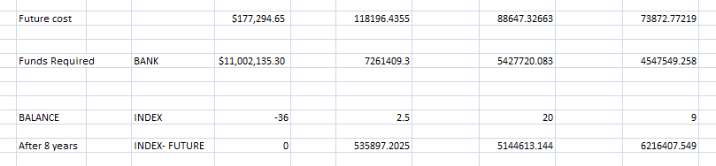
Now, it is super easy to verify all your formulas and even print them if you wish. This way, you can easily find all the errors in your formulas to understand how the numbers are what they are.
10. Maximise the Printing Options When You Are Printing Large Workbooks
Large and widescreen monitors are ideal for working on spreadsheets. However, sometimes, you naturally need to take a printout of your workbook. You need to be especially careful in this case, or you can end up wasting a considerable amount of paper by printing something that will mostly be unreadable and illegible.
This is where Excel comes into the picture, allowing users to adjust the page orientation and size using the Backstage printing options. It is recommended to print spreadsheets on legal-sized paper and in landscape orientation so that every word on the spreadsheet/printout is legible and you do not waste any extra or unnecessary paper.
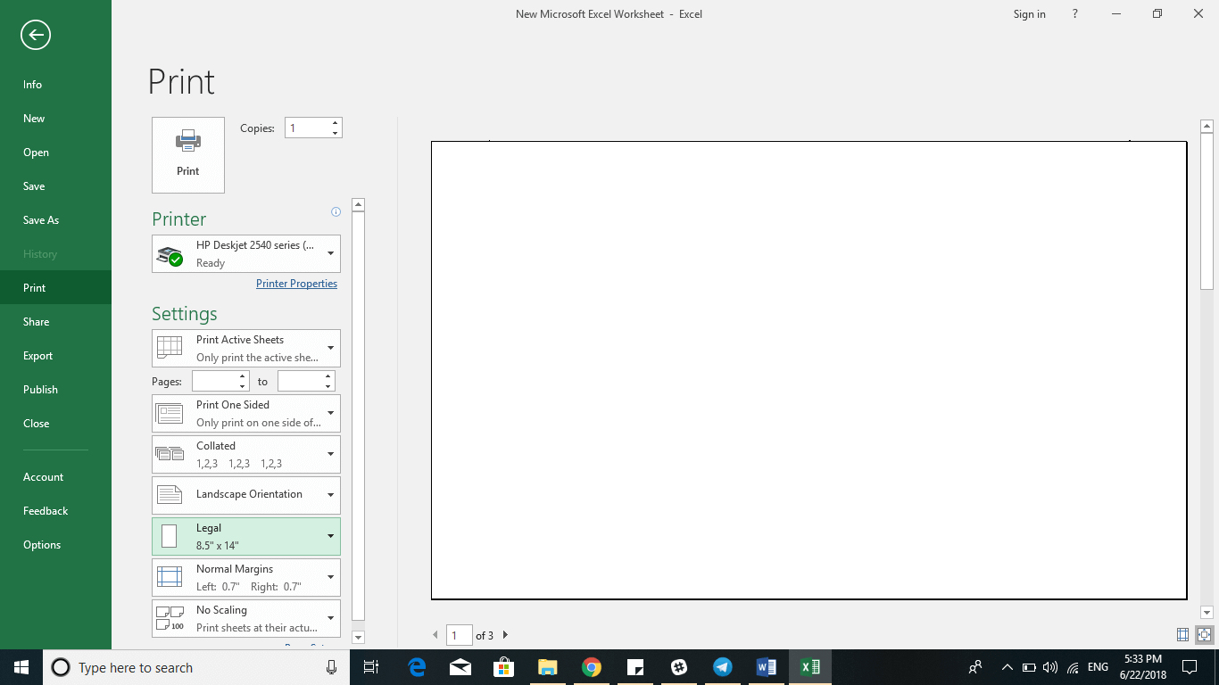
You can also adjust the margins if you wish to fit in any additional details or information on a single sheet. To do that, you can click on the Show Margins tab that is present on the right-hand side of the tab that says backstage print.
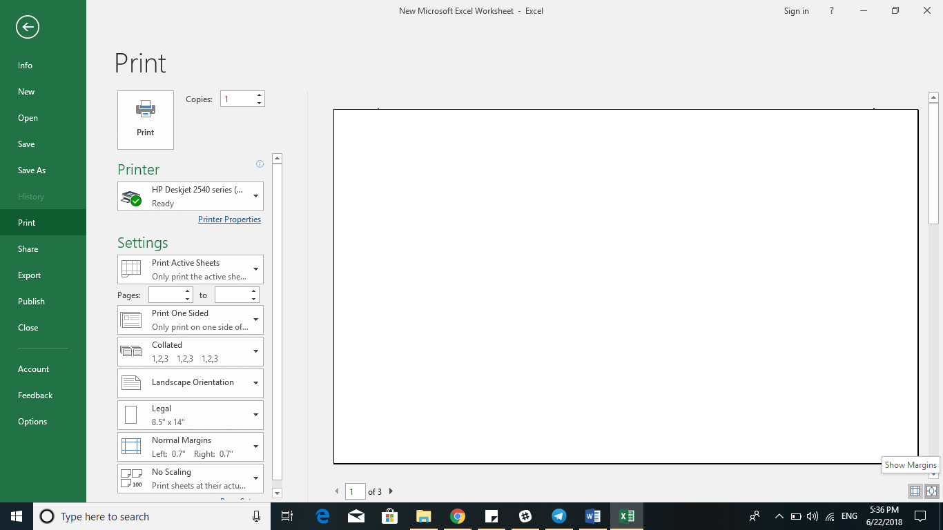
Then you can adjust the margins to your preferences to accommodate any spillover data so it all fits on a single page.
If you are finding it challenging to provide everything on a single page, you can also go to Page Setup at the bottom of the page to make additional adjustments. You can reduce the text size or use the scaling menu to make further changes so that the text is neither too small nor illegible.
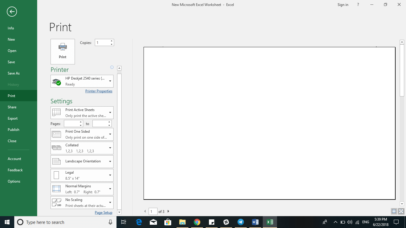
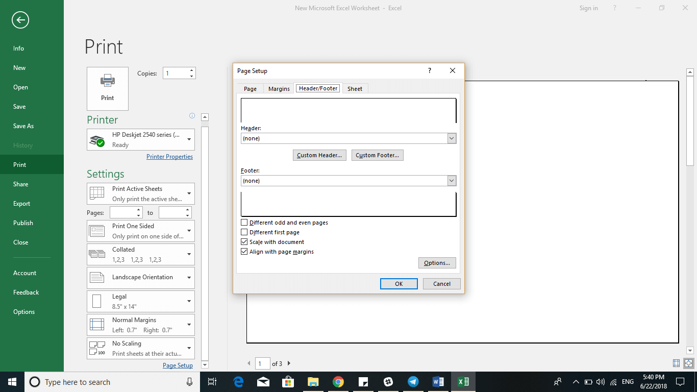
You can also dress your print page with headers and footers using the same dialogue, if desired.
11. Select All with One Click
We saved the best for the last! For beginners who are relatively new to Excel, this will be a lifesaver!
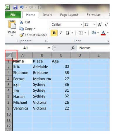
Everyone probably knows that you can select all the text on a spreadsheet by hitting the Ctrl + A shortcut at the same time! But did you know that clicking the corner button, as shown in the screenshot, can select all the data you’ve entered within seconds?
Bottom Line
Microsoft Excel is a treasure trove of tricks and tips that are bound to surprise seasoned users and substantially assist users with beginner-level Excel skills in using this handy tool. Furthermore, you can also use the Excel app on your smartphone for easy access to all your spreadsheets in the Drive.
To learn more about Excel, you can check our Excel training courses.
