
XLOOKUP is an Excel function that searches a range or array and returns a matching value. It replaces VLOOKUP and HLOOKUP: it looks in any direction, returns an exact match by default, doesn’t break when you insert or move columns, and can handle a “not found” message on its own. If you know VLOOKUP, XLOOKUP does the same job with far fewer headaches.
This guide walks through the syntax and the most common real-world uses, with copy-ready examples.
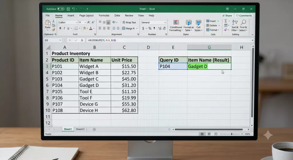
What does XLOOKUP do?
XLOOKUP takes a value you want to find, looks for it in one list, and returns the matching item from another list. For example, you have a product code and you want the matching price, or an employee name and you want their department. XLOOKUP finds the code or name and hands back the value sitting alongside it.
It was released to replace the older VLOOKUP and HLOOKUP functions and is available in Microsoft 365, Excel 2021, and Excel for the web.
XLOOKUP syntax
=XLOOKUP(lookup_value, lookup_array, return_array, [if_not_found], [match_mode], [search_mode])- lookup_value — what you’re searching for (for example, a product code).
- lookup_array — the list to search in.
- return_array — the list to return a result from.
- [if_not_found] — optional text to show if there’s no match (for example, “Not found”).
- [match_mode] — optional: 0 = exact (default), -1 or 1 = next smaller/larger, 2 = wildcard.
- [search_mode] — optional: 1 = first to last (default), -1 = last to first.
The first three arguments are all you need most of the time.
How to use XLOOKUP: a basic example
Say column A has product codes and column B has prices. To find the price for the code in cell E2:
=XLOOKUP(E2, A2:A100, B2:B100)XLOOKUP looks for the value in E2 within A2:A100 and returns the matching price from B2:B100. No column-counting, no sorting required.
How is XLOOKUP different from VLOOKUP?
Four practical differences make XLOOKUP the better choice:
- It searches in any direction. VLOOKUP can only return values to the right of the lookup column. XLOOKUP can return a value from a column to the left just as easily.
- It defaults to an exact match. VLOOKUP defaults to an approximate match, a classic source of silent errors. XLOOKUP is exact unless you tell it otherwise.
- It doesn’t break when columns move. VLOOKUP uses a column-index number, so inserting a column breaks the formula. XLOOKUP references the return column directly, so it keeps working.
- It handles “not found” on its own. No need to wrap it in IFERROR; use the built-in if_not_found argument.
Common XLOOKUP examples
Return a value from the left
=XLOOKUP(E2, B2:B100, A2:A100)Here the lookup list (B) sits to the right of the return list (A). VLOOKUP can’t do this without a workaround; XLOOKUP doesn’t care about order.
Show a friendly message when there’s no match
=XLOOKUP(E2, A2:A100, B2:B100, "Not found")If the code in E2 isn’t in the list, the cell shows “Not found” instead of the #N/A error.
Approximate match (for banding, tax brackets, commission tiers)
=XLOOKUP(E2, A2:A100, B2:B100, , -1)Match mode -1 returns the next smaller item if there’s no exact match, ideal for grade bands or pricing tiers.
Match on multiple criteria
=XLOOKUP(1, (A2:A100=E2)*(B2:B100=F2), C2:C100)By multiplying two conditions together, XLOOKUP finds the row where both are true, for example the right price for a specific product and region.
Return an entire row or column
Because XLOOKUP returns an array, you can hand back a whole record:
=XLOOKUP(E2, A2:A100, C2:F100)<br>This returns all of columns C to F for the matched row in one formula (spilling into adjacent cells).
When should you still use something else?
XLOOKUP covers the vast majority of lookups. For very large models where you’re doing thousands of two-way lookups, INDEX/MATCH or a data model in Power Pivot can be more efficient. And if you’re on an older version of Excel (2019 or earlier), XLOOKUP isn’t available, so you’ll fall back to VLOOKUP or INDEX/MATCH.
Practice makes it stick
XLOOKUP is one of those functions that clicks the moment you use it on your own data with someone to guide you past the edge cases. That hands-on practice is exactly how our Excel courses are built: you work through real examples with a certified trainer, then keep the course manual and free email support afterward.
Ready to master Excel’s most useful functions? Explore our instructor-led Excel training courses, available in-class in Sydney and Melbourne or Online Live across Australia.
Frequently asked questions
For most tasks, yes. XLOOKUP searches in any direction, defaults to an exact match, doesn’t break when columns are inserted, and can return a not-found message without extra functions. VLOOKUP still works, but XLOOKUP avoids its common pitfalls.
XLOOKUP is available in Microsoft 365, Excel 2021, and Excel for the web. It is not available in Excel 2019 or earlier.
Yes. Multiply the conditions together inside the lookup argument, for example =XLOOKUP(1, (A:A=E2)*(B:B=F2), C:C), to match on two or more criteria at once.
Yes. Because it returns an array, pointing the return argument at multiple columns (for example C2:F100) returns the whole matched record, which spills into the neighbouring cells.
It means no match was found. Add a fourth argument to handle it gracefully, for example =XLOOKUP(E2, A2:A100, B2:B100, “Not found”).
