
Slicers are special field filters that can be applied to Excel tables. They are most useful for further dissecting an existing PivotTable report in a worksheet. Slicers are actually graphics objects comprising of a rectangle and special filter buttons. Slicers are inserted into the worksheet from the Slicer command on the INSERT tab of the ribbon.
Steps to create slicers
STEP 1:
Click anywhere in the PivotTable within the worksheet
STEP 2:
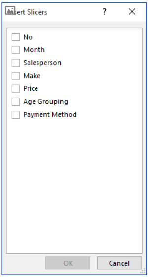
Click on the Insert tab, then click the Slicer in the Filters group to display the Insert slicers dialog box
This box shows a tick box next to each of the fields from the data source…
STEP 3:
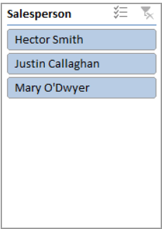
Click on the tick box for Salesperson and click on [OK] to display a Slicer box with the salespeople in it.
STEP 4:
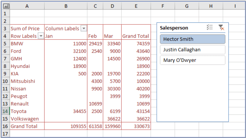
Click on Hector Smith to see only the sales made by Hector Smith OR click on Mary O’Dwyer to see only the sales made by Mary O’Dwyer.
STEP 5:
Click on Clear Filter in the Slicer box to see all of the sales again
For Your Reference…
To insert a slicer into a PivotTable:
- Click anywhere in the PivotTable
- Click on the INSERT tab and click on Slicer in the Filters group
- Tick the field(s) to slice and click on [OK]
Handy to Know:
You can filter on more than one field. To do this click on the first sample, then hold down the ‘Ctrl’ button on your keyboard and click on subsequent samples.
The slicer topic is covered in our Advanced Excel course
Dynamic Web Training is Australia’s leading provider of instructor-led software training.