
Various Excel functions can save a lot of time, as their implementation delivers fast results. Moreover, they are efficient. It is especially useful for data analysis when you have a broad dataset to analyse and make a decision.

We know that Microsoft Excel offers an extensive range of functions, arrays, and visualisations that empower you to rapidly derive insights from data that would otherwise be hard to perceive.
Every SEO and marketer must know how powerful Excel is when it comes to using its functions. It is not necessary to memorise these functions to use them, but you should know when and where a particular Excel function should be used.
It would help you work more efficiently and prove economically beneficial. Now, let’s have a look at the 7 most useful Excel functions for data analysis:
Functions for Data Analysis
1. Find & Replace:
In data analytics, the Find and Replace function has become a go-to tool. Though it may seem conventional, the function accomplishes what it means, i.e., finds text, and then replaces it with some other text entered by you.
This Excel function removes AdWords markup from a list of keywords so SEO can use them directly. Moreover, it can replace all references to a previous month and update the report to the present month.
The Excel function is handy for updating a directory of folder structures for a redirect plan, and it can also update portions of title tags or meta descriptions. If you wish to change HTTP URLs to HTTPS in the URL list, this Excel function is useful. It can also eliminate extra spaces or an incorrect brand name inside a list.
From the Home ribbon, go to the Find & Select option. Now choose Replace, then in the dialogue box that appears, click Options. The dialogue box below will appear.
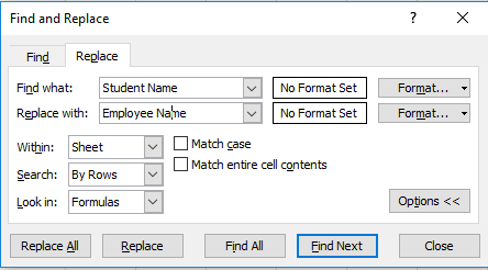
Enter the values you want to replace in the Find what box and the new value in the Replace with box. You can choose Replace or Replace depending on your needs. Excel will smoothly do the needful.
2. Remove Duplicates:
A data analyst usually spends a lot of time integrating data from different sources and pieces of information.
For keyword research, more than five data sources may be needed to generate keyword ideas, and some of these may include overlapping keywords. For that, you can make use of this built-in function to remove the duplicates.
To use this function, you need to highlight the data you wish to delete. Make sure to cover the entire data set and select only the columns that contain duplicates.
Moreover, you have other columns of data matched to the duplicates, which you do not wish to modify. To get an estimate of them, you can utilise conditional formatting to emphasise the clones first.
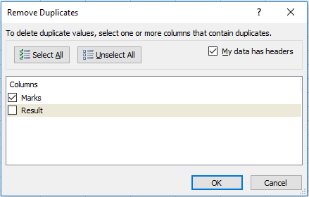
Go to the Remove Duplicates option in the Data tab. Choose the columns you wish to delete duplicate values from, as shown below.
3. Conditional Formatting:
The importance of conditional formatting for analysing or reporting data is unique. You can use this Excel function to highlight good data, bad data, percentage (%) of change, duplicate values, top search volume keywords, and many more.
As shown in the dialogue box below, you can format a particular cell or range of cells with a special formatting effect. You need to practice this Excel function a lot to perceive how powerful it is.
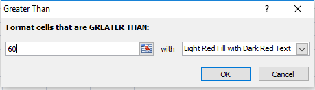
First, select a specific column whose data you wish to format conditionally. Now, go to the Conditional Formatting option from the Homepage ribbon. Then choose Highlight Cell Rules and select the Greater Than option, and the following dialogue box will appear.
Pick the cell with the condition. For example, condition the cell to format with a colour if its value is greater than 60.
4. Filter & Sort:
Filtering and sorting are common Excel features, and their use remains in demand. Occasionally, it happens that SEO can become overpowering, and there arises the need to pair the data with the purpose to prioritise. Under such cases, Filter and sort are useful.
Filtering is particularly helpful when reviewing an extensive dataset and organising it by standard terms.
To understand its usefulness, you can create a list of keywords and then filter by how many of them include identical topic keywords.
Sorting is helpful when you want to prioritise a list by its lowest or highest values. You can sort landing pages by highest revenue, lowest conversion rate, or a maximum number of sessions to prioritise where to concentrate your efforts to improve.
With advanced sorting, you can seamlessly sort by keywords with the highest search volume and lowest competition, or by landing pages with the most sessions but the lowest conversion rate.
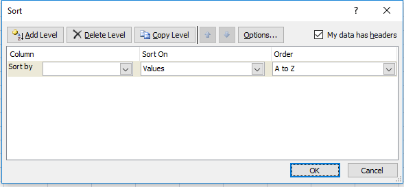
First of all, select a particular column whose data you wish to sort. Now, go to the Sort & Filter option from the Homepage tab. Then choose Custom Sort, and you would see the following dialogue box.
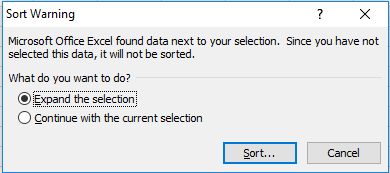
Now, click on the Sort option, the following dialogue box will open. Select how you wish to sort by and choose Order, i.e., A to Z or Z to A. Also, select the right option in the Sort drop-down menu, as per your needs.
5. LOWER(), UPPER() and PROPER():
The three Excel functions – LOWER(), UPPER(), and PROPER()- are used to modify text to lowercase, uppercase, and sentence case (in which the initial letter of every word is capitalised).
When data analysts work with large volumes of data, the need often arises to convert text to upper or lower case or to change sentence case. Under such circumstances, these functions are handy. Let’s have a look at its syntax:
Syntax: =Upper(Text)/ Lower(Text) / Proper(Text)
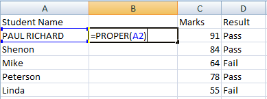
For instance, in the example below, insert a temporary column adjacent to the column containing the student name if you want to convert the name of a particular student to proper case.
Now, in cell B2, type
=PROPER(A2)
, and then press Enter.
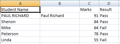
You would see that the student’s name changed to proper case, as shown below.
In the above example, to convert the text to lowercase, you have to type =LOWER(A2) instead. To turn the text to upper text, use
=UPPER(A2)
6. Recoding & Frequencies:
The if function allows you to place a condition for Excel to execute. The function is very helpful if a date needs to be recorded. For instance, in the dataset, if you want to identify the most commonly ordered fabric, you can use the statistical function MODE. However, the function has a limitation – it only works on numbers, not on text. You will get an #N/A error if you apply it to the text. When you convert the fabrics to numbers, you can effortlessly obtain the answer. To see the results, you can use the if function. The basic syntax is:
=IF(logical_test, [value_if_true], [value_if_false])
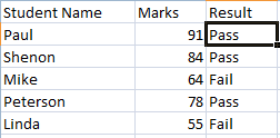
If you had marks in cell C2, and you wish to test these marks to analyse if they are at least 70, then you can use the IF function in this way:
=IF(C2>=70, “Pass”, Fail”)
7. CONCATENATE():
This Excel function is useful for combining text from two or more cells into a single cell. The need to merge data from different cells into a single cell frequently arises in data analysis; the function works like a charm in these situations.
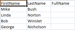
Suppose you wish to concatenate the first name and last name of a person to the full name, as shown in the figure below. You can do that by using the concatenate function.
Syntax:
=concatenate(text1, text2, …, textn)
If you want to merge content in cells A1 and B1, then use this:
=concatenate(A1, B1)
and copy it.
To learn more about Excel, you can check our Excel courses.