How to Create Pivot Tables in Excel 2016 - Dynamic Web Training Blog

Microsoft pioneered an excellent tool to create, analyze, store and manipulate data. We know it by the name of Microsoft Excel and true to its name; it is one of the greatest spreadsheet application in the Microsoft Office suite.

How to Create Pivot Tables in MS Excel 2016 with Ease - Dynamic Web Training — Click image to enlarge

Initially, it worked fine from evaluating simple expenses for analyzing complex data. Today, the latest version – the Microsoft Excel 2016 is an excellent option but also potent tool for data analysis for business insights and watching trends.

For making better rational decisions, you not only need to process data quickly but also effectively. But the rapid accumulation of data can become overwhelming and can leave you gasping. In no time, you may feel lost, and you have a burden of extensive data to compile.

The magic lies in this Excel tool with one of its features like Pivot Table coming to play. It helps you exploit and play with the data stored in the cells. Pivot tables will help you utilize its prowess of data analysis, exploration and summarization to present it in a manner which is easy to comprehend.

What is a Pivot Table?

As said earlier, a pivot table in MS Excel is a tool to summarize, explore and analyze massive scattered data. The summarization takes just a few clicks, and the results are there for your comprehension.

The pivot tables are flexible and can be modified or presented at your choice. You can customize and adjust the way you want, and for as many cells you want. It is ideal for calculating, evaluating and displaying information in tables and breakdowns to the scale you need.

Pivot charts can also be created based on pivot tables. These charts will automatically be updated when your pivot tables get updated. Many times it can unravel the hidden facts buried under your data.

The images shown below is a pivot table and a pivot chart –

What is a Pivot Table 1 - Dynamic Web Training — Click image to enlarge

What is a Pivot Table 2 - Dynamic Web Training — Click image to enlarge

How to create a Pivot Table?

Prerequisites

The data in the sheet should be in a tabular format, and no blank row or blank column should be left.
Data Types of the data in the columns should be the same. You should not mix numbers, date, currency, and text in a single column
If you alter data in your Pivot Table, your actual data will never be changed as Pivot Table works as a snapshot of the original data.

Steps:

Creating Pivot table is very easy, you need to follow the below steps –

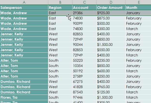
Select the table of data or cells from your data table. The cells should include the headers. You can select the entire table or some cells from the table to create a pivot table.

Pivot Table Step 1 - Dynamic Web Training — Click image to enlarge

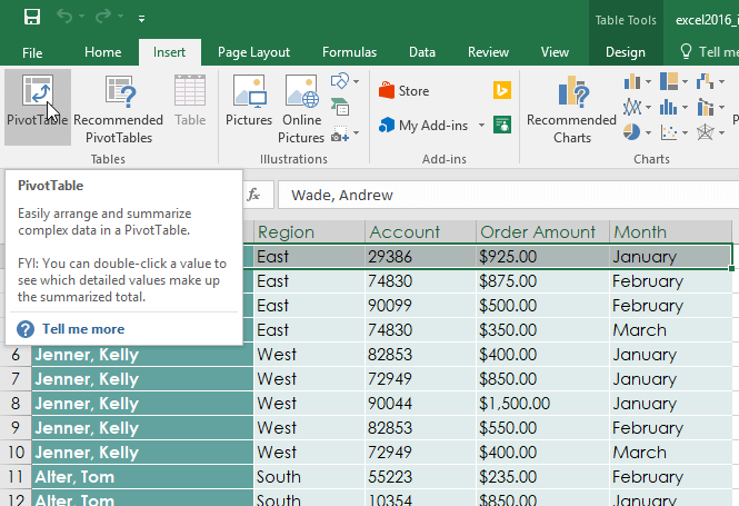
Now to go Insert tab and click on Pivot Table.

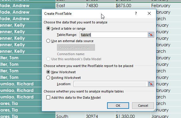
Pivot Table Step 2 - Dynamic Web Training — Click image to enlarge

Next, you need to select your data source and settings in the Create Pivot Table dialogue box and then click OK. It will place your Pivot Table in a new worksheet. You can give a name to the table. In our example, it is Table1.

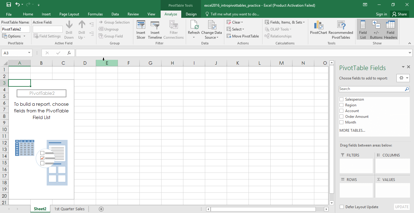
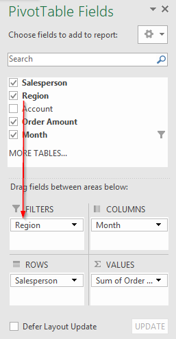
Pivot Table Step 3 - Dynamic Web Training — Click image to enlarge

Now the PivotTable options will be opened. You can select which PivotTable Fields you want to keep in your PivotTable. The fields that have numeric value can be dragged to the Values column to get the average or totals.

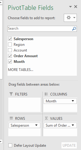
Pivot Table Step 4 a - Dynamic Web Training — Click image to enlarge

Like in our example we want to see which salesman has how much order amount each month. So, we select our fields as shown –

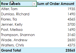
Pivot Table Step 4 b - Dynamic Web Training — Click image to enlarge

This gives a PivotTable like this –

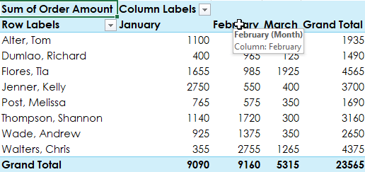
Pivot Table Step 4 c - Dynamic Web Training — Click image to enlarge

The selected and checked fields add to the Row, and if you want to see a specific field in the column as we did, you need to drag it to the Column area below.

You can sort the data as a regular Excel table in the Pivot Table

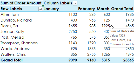
Pivot Table Step 5 - Dynamic Web Training — Click image to enlarge

The columns with the data for each row will be updated and refreshed according to the Rows.

You can select or deselect some rows from the table as per your requirement.

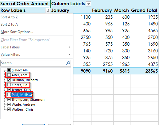
Pivot Table Step 6 a - Dynamic Web Training — Click image to enlarge

Here we have deselected the three rows from the table, and we get the table without these rows when we click on OK.

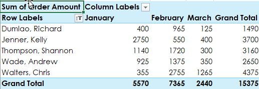
Pivot Table Step 6 b - Dynamic Web Training — Click image to enlarge

Similarly, you can omit some columns as per your choice from the table and see the data without those columns –

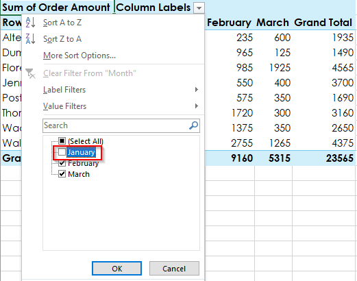
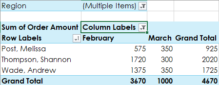
Pivot Table Step 7 a - Dynamic Web Training — Click image to enlarge

We have unchecked January from the table, and we can see data for only February and March in the table –

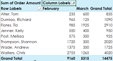
Pivot Table Step 7 b - Dynamic Web Training — Click image to enlarge

The PivotTable Fields can also add a filter to the table. In the example, we have added the Region field in the FILTERS.

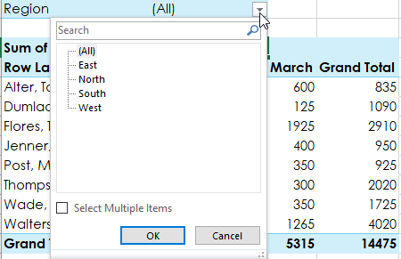
Pivot Table Step 8 a - Dynamic Web Training — Click image to enlarge

Filter for Region has appeared here-

Pivot Table Step 8 b - Dynamic Web Training — Click image to enlarge

Now, suppose we want to see data for only East and North region, we can uncheck the South and West regions from the filter and click OK.

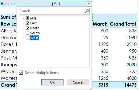
Pivot Table Step 8 c - Dynamic Web Training — Click image to enlarge

So, the data has been filtered for only East and North regions –

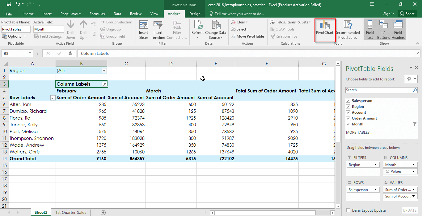
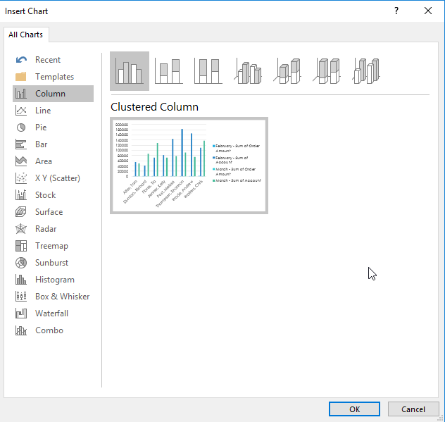
Pivot Table Step 8 d - Dynamic Web Training — Click image to enlarge

You can create Pivot chart from the pivot table, through Pivot Chart optionWhen we click on the Pivot Chart option, Insert Chart dialogue box gets opened. You can select chart type as per your need from the window. In our example, we are choosing the clustered column chart. If you hover on the chart type, you’ll get to see a small preview of how your chart will look-

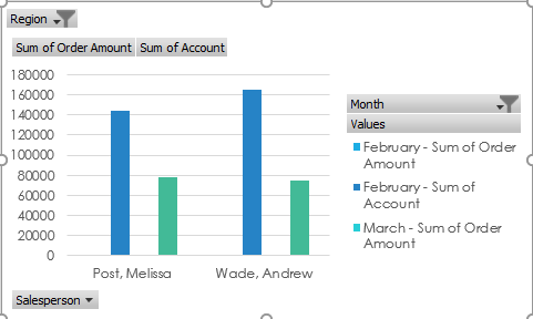
Pivot Table Step 9 a - Dynamic Web Training — Click image to enlarge

Pivot Table Step 9 b - Dynamic Web Training — Click image to enlarge

Upon clicking OK, it creates a Pivot Chart or a graphical representation of your Pivot Table. You can drag and drop the chart at any place you want on the sheet. You also can increase or decrease the size of the chart quickly.

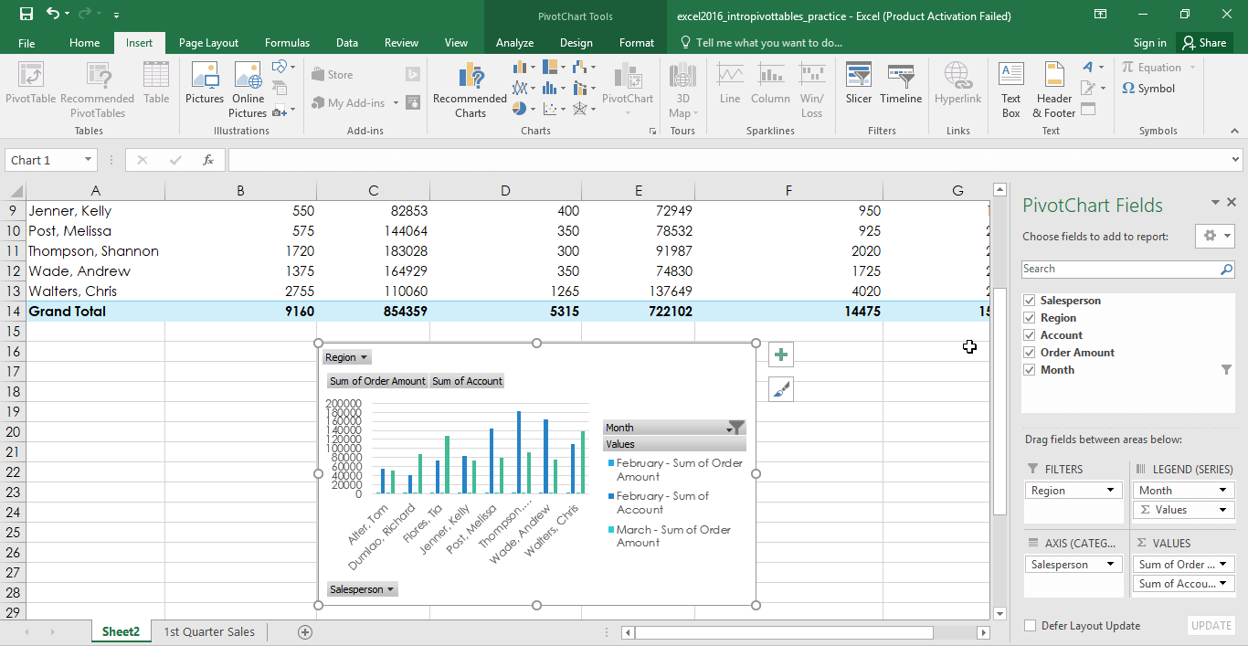
Pivot Table Step 9 c - Dynamic Web Training — Click image to enlarge

You can manipulate the fields on the chart, adding filters

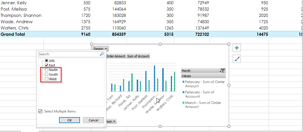
Pivot Table Step 10 a - Dynamic Web Training — Click image to enlarge

In our example, we have unchecked the North, South and West regions. The graph is now showing us data according to East region only.

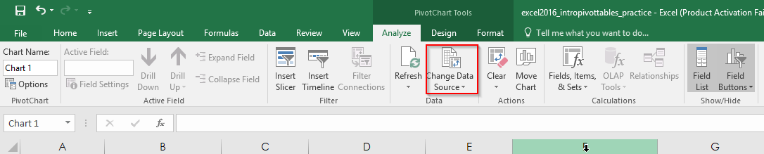
Pivot Table Step 10 b - Dynamic Web Training — Click image to enlarge

You can have different tables on different worksheets. You can change the source of your Pivot Table through the Change Data Source option.

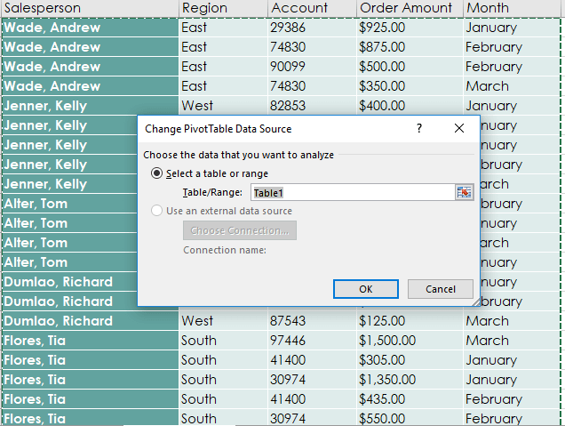
Pivot Table Step 11 a - Dynamic Web Training — Click image to enlarge

Pivot Table Step 11 b - Dynamic Web Training — Click image to enlarge

You can provide the Table name that you want to add as a new data source –

What is a Recommended Pivot Table?

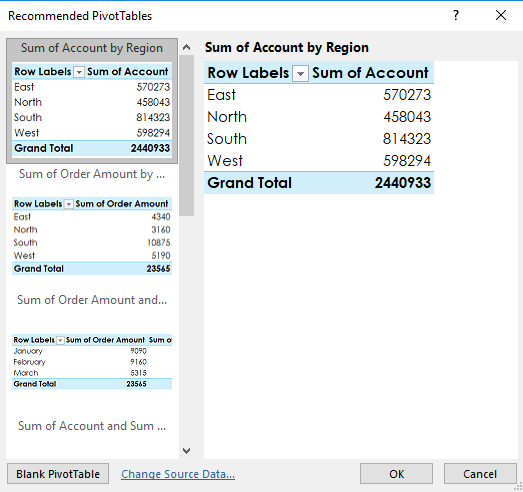
Pivot Table Step 12 - Dynamic Web Training — Click image to enlarge

Recommended pivot table option enables you with an automatic pivot table. This option provides a template for creating Pivot Table. You can select any one of the types, change source data or create a blank pivot table in the Recommended Pivot Table Dialogue Box.

Recommended Pivot Table is an excellent functionality for those who have insufficient knowledge about Pivot Tables. After you created the recommended Pivot Table, you can then manipulate the filters like the Pivot Table you create manually. You also can change different orientations.

How to remove a Pivot Table?

If you do not need the Pivot Table anymore, you can select the entire table and press Delete. Make sure the whole table is selected; otherwise you’ll get an error message – “Cannot change this part of a table Report.

Final Words:

Create your tables in a manner of how you want your data to be displayed. Utilize the PivotTables and make your process simple. Invest your time and practice using the pivot tables and its uses and various data types.

What is a Pivot Table?

How to create a Pivot Table?

What is a Recommended Pivot Table?

How to remove a Pivot Table?

Final Words:

By Dynamic Web Training