Finance professionals or those handling student databases are often faced with the challenge of searching through a vast data pool, to find the data of their choice. If you too get goosebumps when asked to look for a specific data, from an overwhelming amount of data stored on an excel sheet, then here’s a secret treat for you.

VLOOKUP and HLOOKUP
VLOOKUP and HLOOKUP are two powerful functions in Microsoft Excel that allow you to use a specific section of your excel spreadsheet, to search for the correct data. These functions let you search through the excel table containing data, based on user’s requirement and extract the appropriate result from the table.
In simple words, consider an excel sheet with names of 100 employees in column one and their corresponding details like ID, department, designation, etc. in the next 10 columns. Now, imagine a situation where you have been asked to prepare a sheet of 30 random employees out of 100 employees and are required to display their corresponding values from only 4 out of the 10 employee detail columns present in the excel sheet.
You can either choose to take the tedious way and manually search through the sheet for every employee name & then search for the required corresponding values in respective columns or use VLOOKUP or HLOOKUP function.
Before we can go into the formation and actual usage of these two powerful functions in excel, let’s get a basic understanding of these two powerful functions first:
VLOOKUP
As the name suggests, the “VLOOKUP” (where V means vertical) function in excel is used to look across a set of values placed vertically or in columns in an excel worksheet. It means that each column is responsible for one unique kind of data.
For Eg: Consider a simple table containing student details like – Student Enrollment Number, Student Name, and Percentage. Here, there would be a separate dedicated column for only student enrollment numbers, one column for student names and so on.
HLOOKUP
As the name suggests, the “HLOOKUP” (where H means horizontal) function in excel is used to look across a set of values placed horizontally or in rows in an excel worksheet. It denotes that each row is responsible for one unique kind of data.
Consider the same above example, with the data now formatted by rows instead of columns.
Applying VLOOKUP and HLOOKUP Functions
Consider a situation where you have an excel sheet containing 50 rows (each row corresponding with a student detail) and 10 columns (each column containing specific data type). The first column is the student enrollment number, and the rest of the 9 columns have different data types like student name, percentage, etc.
Now imagine that you are required to prepare a report for 5 random students (whose enrollment numbers are provided to you) and you are required to display the names of each of those 5 students. You can either search through the sheet containing 50 rows and 10 columns manually, for every student’s enrollment number & their corresponding names in the respective column or use VLOOKUP function.
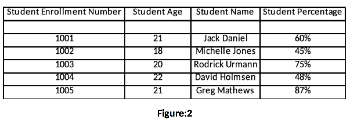
Refer Figure: 2 as the source sheet for this example.
Start by creating a new excel sheet. The first column will be the student enrollment number (with student enrollment number populated) followed by the column for student name for which we need data. It is the column where we shall be applying the VLOOKUP function.
Start by creating a new excel sheet. The first column will be the student enrollment number (with student enrollment number populated) followed by the column for ‘student name’ for which we need data. It is the column where we shall be applying the VLOOKUP function.
Applying VLOOKUP Function
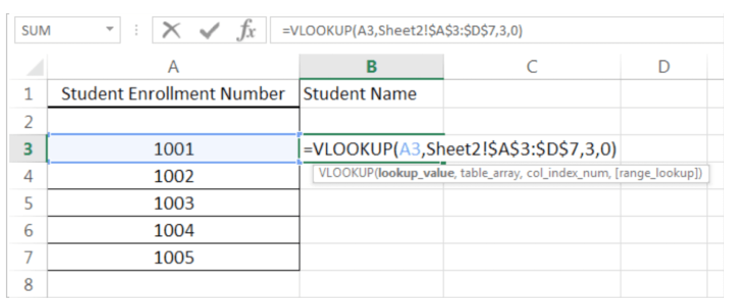
VLOOKUP is represented by the general formula:
=VLOOKUP(lookup_value, table array, col_index_num, [range_lookup])
lookup_value | Will be the cell reference of the cell in which student enrollment number ‘1001’ resides, in the new result/report sheet (A3 in this example). |
table_array | The source of data where you are trying to find the corresponding value (Student name, in this case). In this case, it will be the entire source sheet with 100 rows and 19 columns. |
col_index | This is the most important parameter of the formula. This value is the COLUMN NUMBER from the SOURCE SHEET, where the desired value resides (desired value, in this case, is Student name). Assume that the student name column is the 3rd column in the source sheet, then the col_index_num value will be 3. |
range_lookup | This value is either 1 (True, Approximate match) or 0 (False, Exact match). It is most advisable to select 0, as you would surely not be interested in approximate value, especially when it comes to critical records. |
Thus, the resulting formula for this particular example would be:
=VLOOKUP(A3,Sheet2!$A$3:$D$7,3,0)
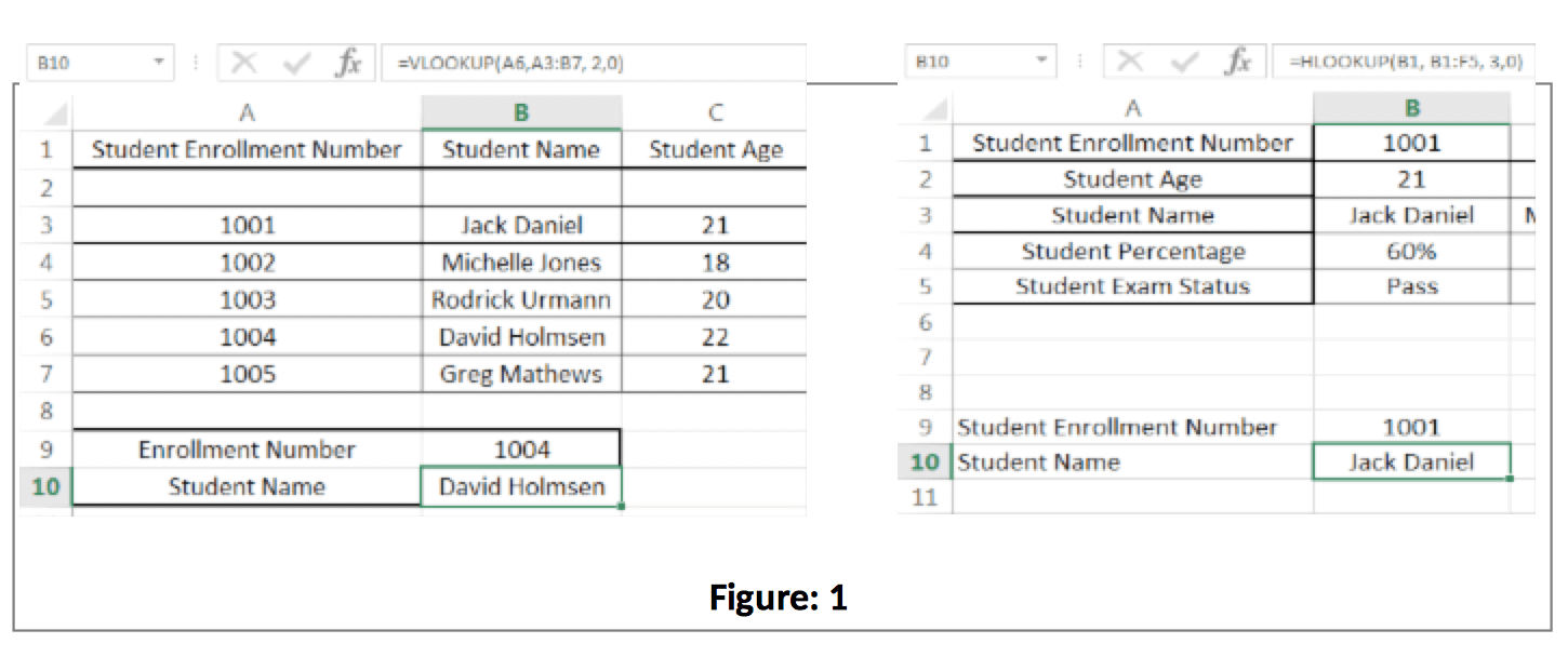
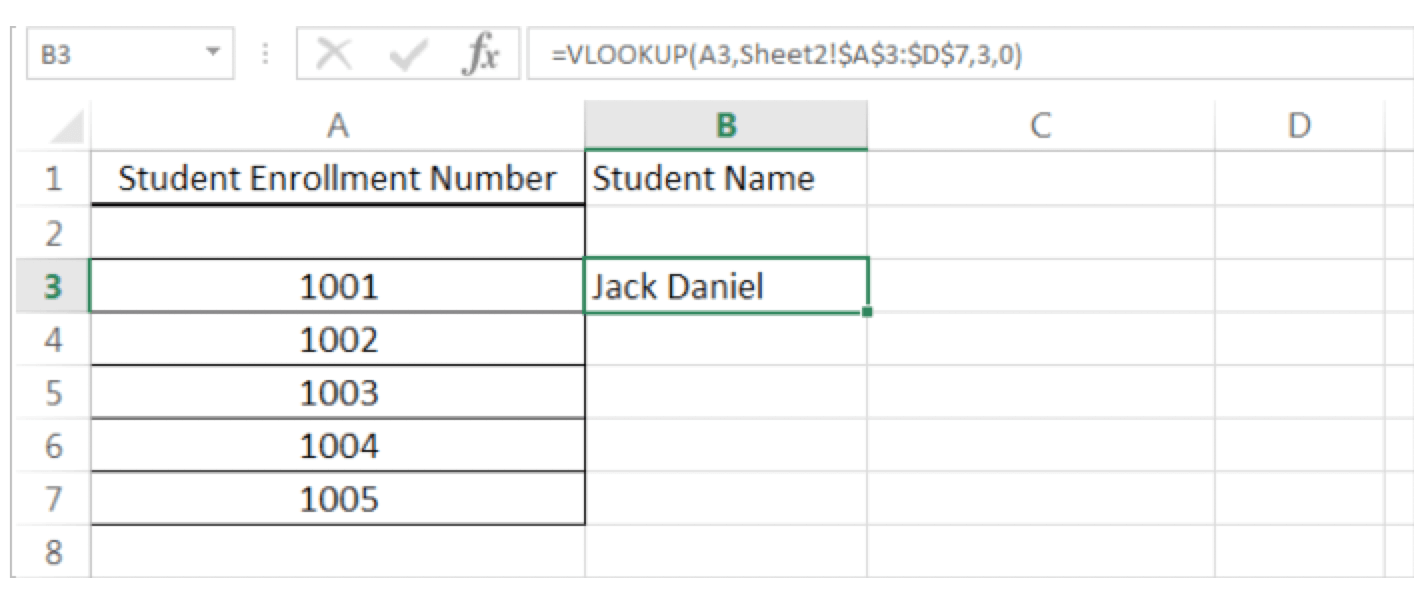
The corresponding name for student enrollment number 1001 will be shown in the desired column as below.
Applying HLOOKUP Function
The HLOOKUP function has almost the same syntax as VLOOKUP. The only exception is that, in HLOOKUP function, these lookup occurs horizontally and thus, you need to specify a row index number instead of column index like in VLOOKUP.
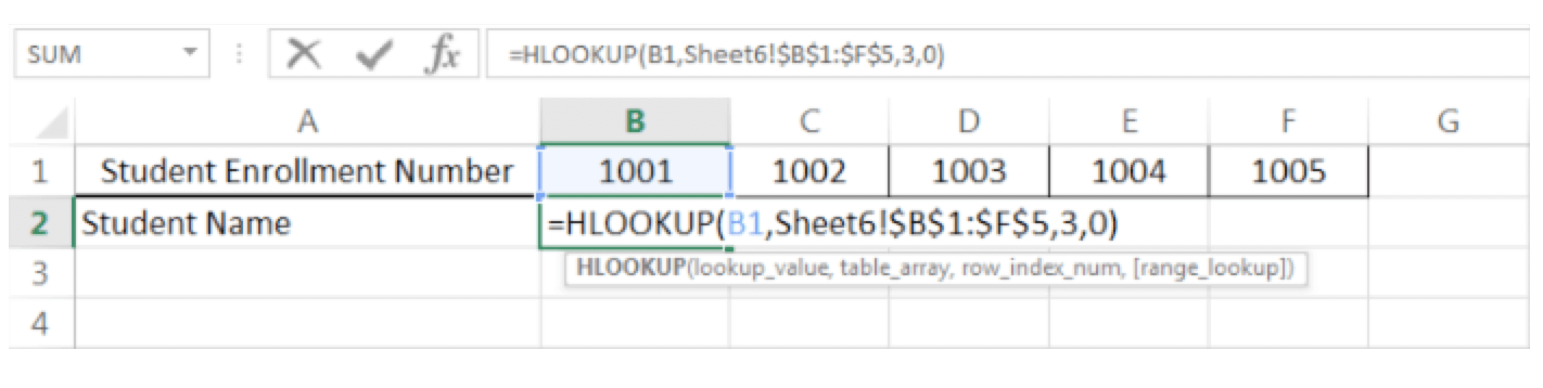
=HLOOKUP(lookup_value,table_array,row_index_num, [range_lookup])
row_index | This value is the ROW NUMBER from the SOURCE SHEET, where the desired value resides (desired value, in this case, is Student name). Assume that the student name row is the 3rd row in the source sheet, then the row_index_num value will be 3. |
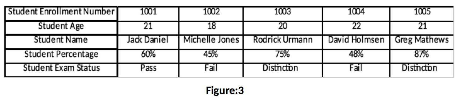
Now consider the same above example, where this time, the data is in rows instead of columns. Thus, now you have an excel sheet containing 50 columns (each column corresponding with a student detail) and 10 rows (each row containing specific data type).
Refer Figure: 3 as the source sheet for this example.
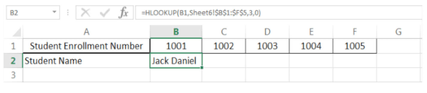
Assume that the first value in front of student enrolment number row is 1001 (reference cell B1). Now, in the second row, we wish to display the name of a student, and so, we will apply HLOOKUP in this row, i.e. ‘Student Name’ rows.
Thus, the resulting formula for this particular example would be:
=HLOOKUP(B1,Sheet1!$B$1:$F$5,3,0)
The corresponding name for student enrolment number 1001 will be displayed in the desired row as below.