
Excel Lookups are great ways to search for a particular value using queries within a large data set. There are many types of Lookups available in MS Excel and each one is having a different use. Among them, Index and Match are considered the most common type of lookup which offers a powerful formula for looking up in excel sheets.
Match in Microsoft Excel
The search mechanism is used in Index and Match is known as a two-way lookup which allows you to do a matrix lookup on the given dataset. This formula may seem a little complex than Vertical Lookup, but when you get to know about the three components and how these formulas are interacting with each other, you’ll love to use it.
When to use Index and Match?
The other name of Index and Match is Matrix Lookup. That means, Index and Match has one condition to work – your data needs to be in a Matrix format. Vertical Lookup and Horizontal Lookup needs to be present in your data. It is the cross-reference in your data for vertical and horizontal fields.
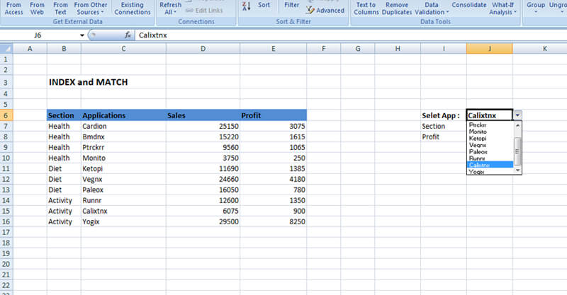
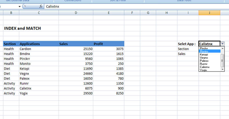
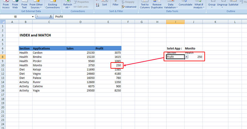
Here is an example of data where you can use Index and Match –
Difference between Vlookup and Index and Match?
Index and Match are considered better than Vlookup. But, why? Let’s see with an example.
In this same example, classical V lookup is not going to work. To make Vlookup work here, the Applications, which are a unique set of data needed to be on the left most column and Section, which are not unique for each set of data needed to be on the right to the Applications column.
So, Vlookup here will not be able to search the value you are looking for. For example, if I am looking for Profit against each unique Section for a selected Application, Vlookup is not good for that. It won’t work, as it is working with three components – Section, Profit, and Sales forming a matrix.
So, if the objective of the above chart is to pull the data like the Sales or the Profit of any particular application we desire. To do such an operation, vlookup will not be able to perform the function. Instead, Index and Match will perform perfectly here.
How do Index and Match work?
With the Index and Match, now, let’s see how this is going to work here.
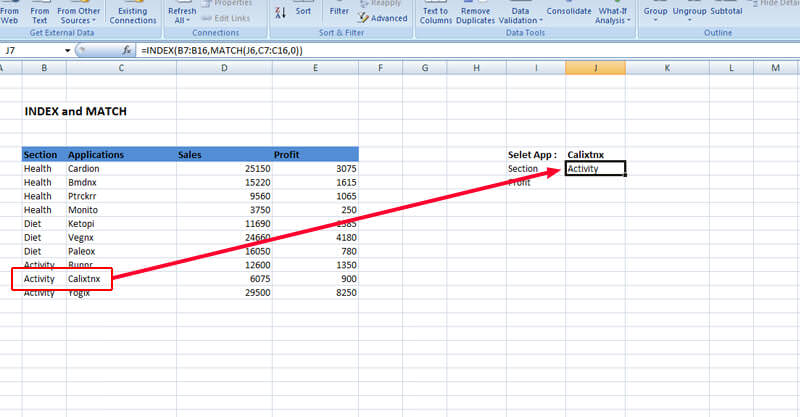
Let’s say we have selected Application- ‘Calixtnx’ in the above example. To understand how Index and Match works, first, we must check out the formula or the syntax –
= INDEX ( array , MATCH ( lookup_value , lookup_array , 0 ) , MATCH ( lookup_value , lookup_array , 0 ) )
So, there are three components in the formula, first, the array which is the base, 1st lookup array, and 2nd lookup array.
Index Functions:
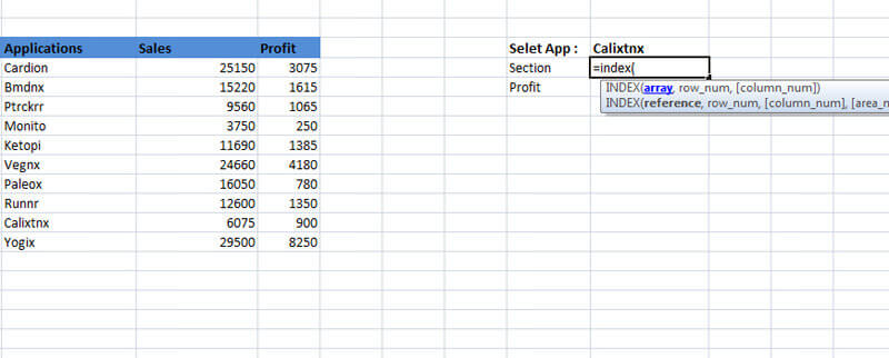
First, we need to see how the index function works. In our example, let’s use the index function in the Section.
When we insert the Index function, we can see the three arguments in the Index function – array, row numbers and column numbers. The column is in square brackets. It means that is an optional argument.
To understand Array, we can think of Index as a GPS function where we have to insert a map (arguments) to find our location. The map here is the array.
First, we highlight the map in the example, which is the first column. We want to see on which section is Calixtnx located.
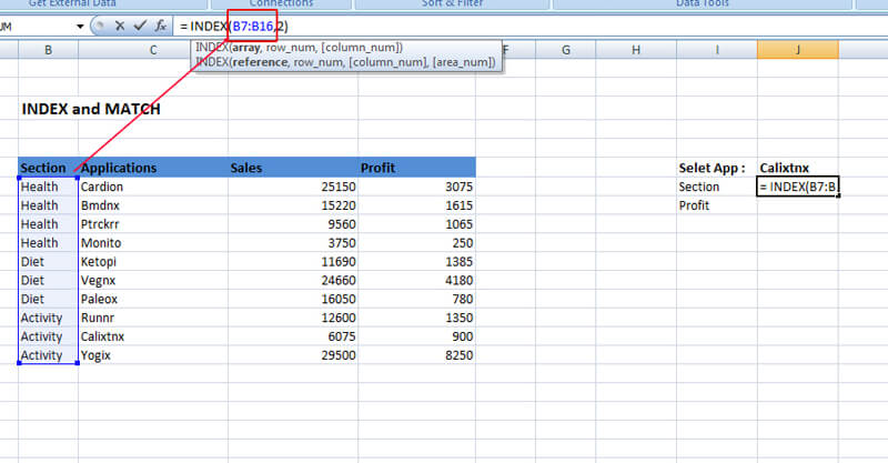
Here we are not looking at the exact answer, with Index function we are only defining the map or the region where our answer lies. It doesn’t matter what you lookup problem is. In this case the answer lies in the Section column. Hence we select the region from B7 to B16.
Now to the next arguments which are the row numbers and column numbers. Let us think of them as the Latitude and the Longitude.
The row numbers define the exact row in the array. Here let us input the row number with 3 in the ‘row_num’ argument and since the Column number is in Square bracket, let us ignore it for no and close the bracket without entering any column number.
The answer it returns is the ‘Health’. Here we actually get a wrong answer as we manually entered row number as 3 instead of 9. But we know one thing for sure the index function is working.
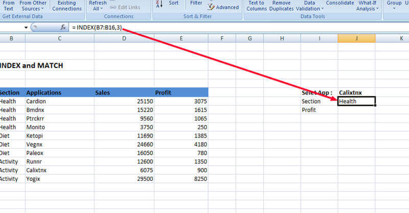
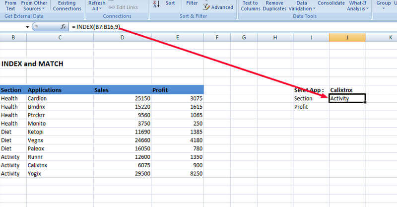
It counts the header in the columns as row 0, as a matrix and then starts counting from 1 through the rows. Therefore, when we put row_num = 3, it gave us ‘Health’ as a result. If you put 9 , it will return with Activity as the Section.
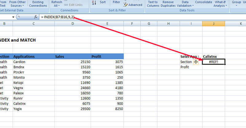
Now, if we put column_num= 1, it still will give ‘Health’ in the Section, as Section is the column number 1. It takes that as a default value. But, if we put column_number = 2, it shows #Ref! in Section, as we are going out of the array (map) we have given to the index(GPS).
This is how the Index function works. But, we do not want to enter numbers directly into row_num and column_num arguments. We want to use the functions which return number value according to the logic of the search we want to put in. To do it without entering the row and column numbers manually, we need the Match function.
The Match Function
We generally use the Match function, with Index function and these two work best together to search for a particular thing in a large dataset. Hence in the formula, Match always needs a lookup value.
Syntax of the Match function is - =MATCH(lookup_value, lookup_array, [match_type]
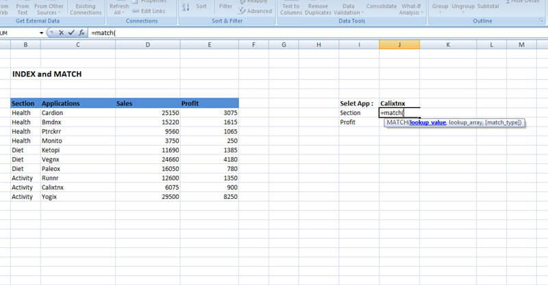
In the lookup_value argument, we enter the data we are looking up. In our example, we’ll enter “Calixtnx”.
Next, we enter the array in which we are looking for ‘Calixtnx’, that is the column 2. In the argument, we’ll enter C7: C16 where we kept our Applications.
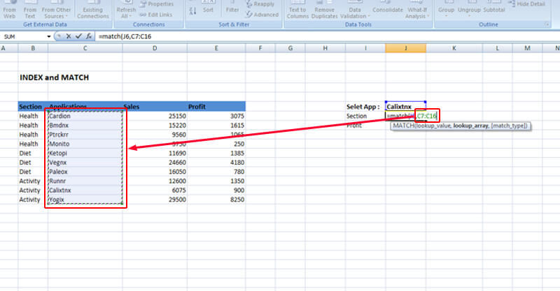
Note: In case of Match function, we need to keep in mind that lookup_array should be linear. It cannot find values present in both directions, i.e., horizontally and vertically.
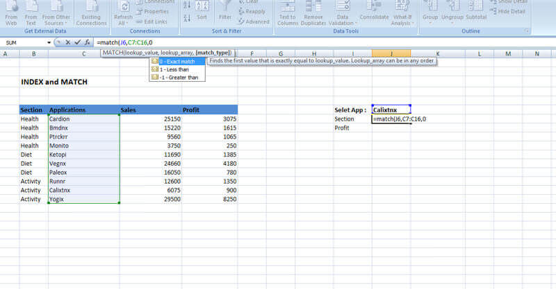
The next argument is ‘match_type’, where we’ll use the Exact Match in the majority of the cases. Greater than or Less Than values are used in some special cases.
So, our function now looks like this –
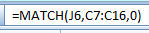
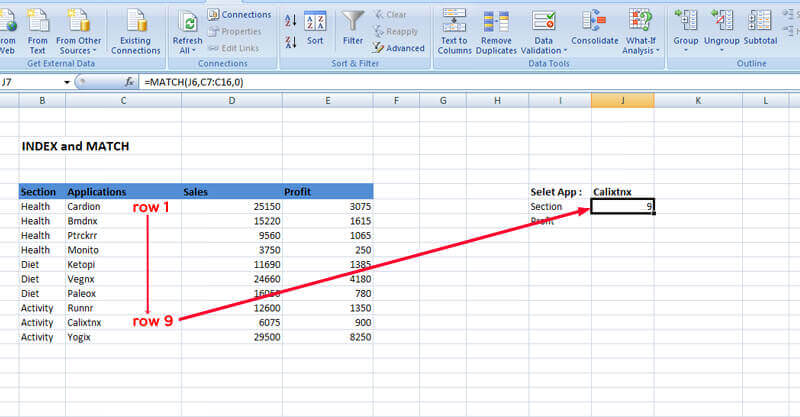
The result we get out of this function is 9. This means ‘Calixtnx’ is in the 9th position in the array. 9th position is C15, which is true.
Index and Match Together
Now, coming to the final stage, we’ll be using both Index and Match functions together. Here we’ll use Match as an argument in the Index function.
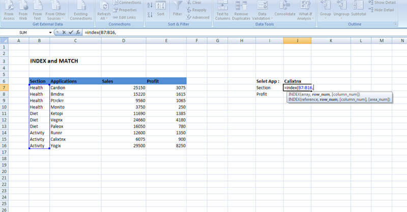
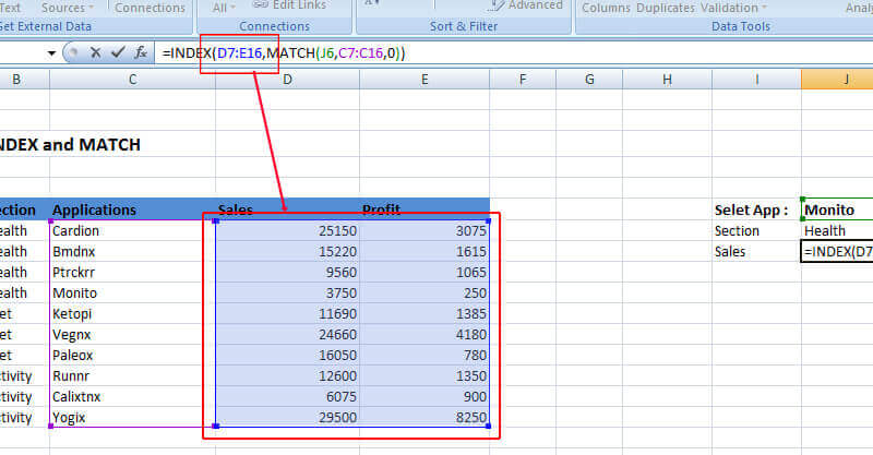
In our example, we’ll use the Section column as an array, i.e., the first argument in the Index function. Therefore, we’ll write the function like =INDEX(B6:B17,…)
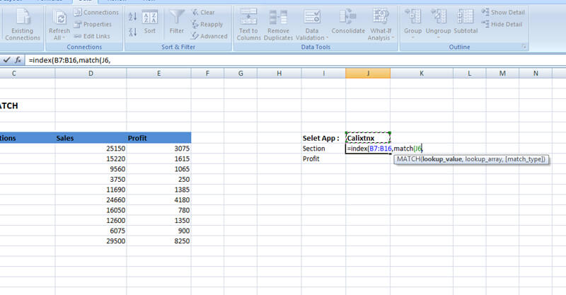
For the second argument ‘row_num’, we’ll use Match function to look up for ‘Calixtnx’ in the Applications column. We’ll write the function like – match (J6,C7:C16,0)
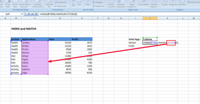
This will give the Section in which ‘Calixtnx’ Applications is used, that is ‘Activity’ as a result.
Note: For using Index and Match function, we need to keep in mind that array for both the functions should be of the same length.
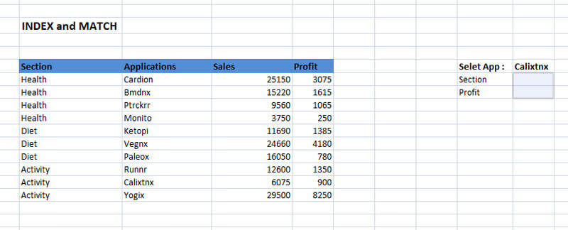
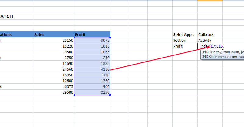
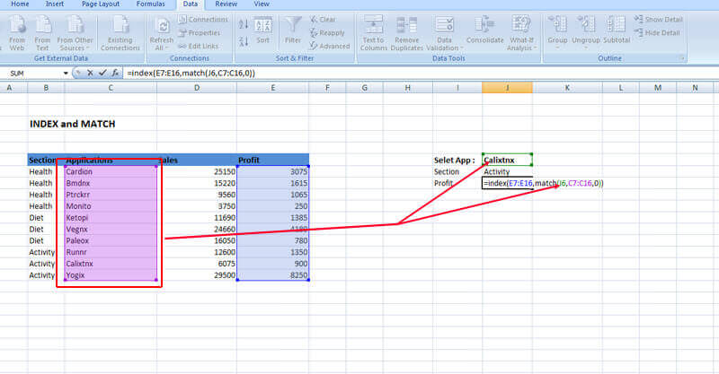
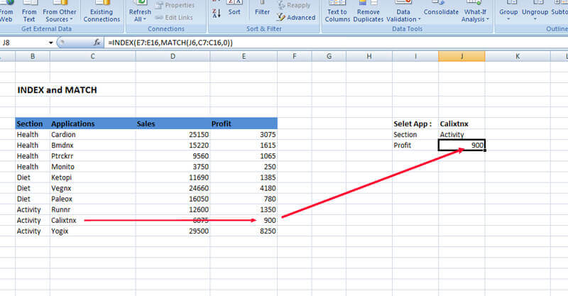
We’ll follow the same technique to find the profit against Calixtnx like the following –
We get the Profit –
Switch between two columns as a result
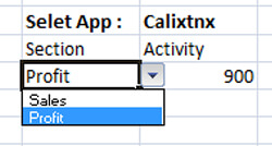
Till now we have seen a simple function in our example. Let’s make it a little complex. Now, we want to switch between Sales and Profit using a dropdown and the value against it should also be changed.
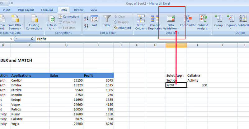
To do that first I am adding a Data Validation operation to create a dropdown which consists of Profit and Sales so that we can switch between them. Select the cell in this case and click Data Validation from the Data Tab.
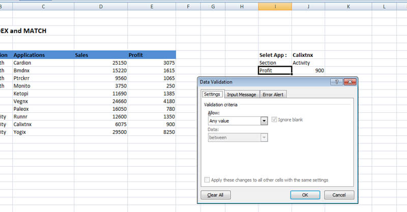
The dialog box of Data validation looks like the picture shown below:
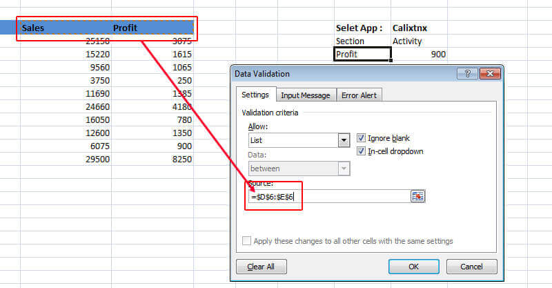
In the Allow Dropdown, Choose List and Select the Sales and Profit Headers as the Source.
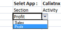
So, we get a dropdown list like this –
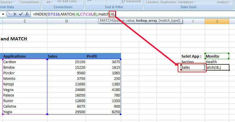
Now, we want the value also gets changed against Profit or Sales, whatever we select. To achieve that, we need to use the Match function again, but now in the ‘column_number’ argument of the Index function, which we did not use in our previous example.
First, we need to update our map that is the ‘array’ argument in the Index function, as now the data we are looking for can be in both Profit and Sales column. Therefore, we’ll include both of them.
Now, we need to check out how many columns we are going to move in and the value depends on what we input. For that, we are going to use again the match function where the lookup_value is where ‘Profit’ or ‘Sales is.
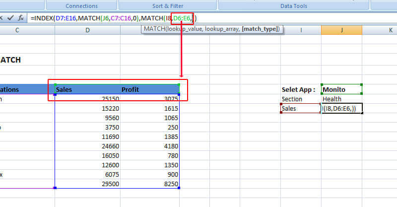
Next thing we have to do is get the value for ‘lookup_array’ argument of the Match function. Our array is in the columns Sales and Profit that starts with D6 and E6. Therefore, here we’ll enter D6: E6 in the argument to get the result.
Lastly, since we are looking for an exact match, we’ll put 0 in the match_type argument as shown below.
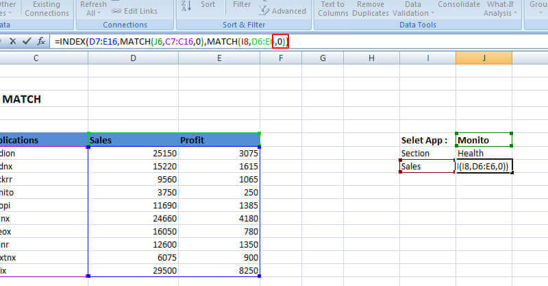
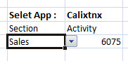
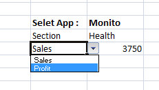
What we get out of this? We can now change the Profit or Sales and we get the value for it-
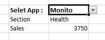
We can add a data validation similarly for the Select App, where we’ll change the Application and we’ll get Section and Profit/ Sales for that Application. For example, we are now selecting ‘Monito’ Application. We’ll see the value changing according to Monito Application.
This is how you can use Index and Match functions in MS Excel for finding the correct value against multiple arguments in a huge number of data that is in a matrix format. They can be used to look up anything against very complex queries as well.
To master the Index and Match and LookUp functions, we recommend our highly-rated Microsoft Excel Training Courses available in-person or online live.