
A Power BI data model or semantic model is the set of tables, relationships, and calculations loaded into Power BI’s in-memory engine. A schema refers to how these tables are organized. It underpins all reports and visuals. A high-quality model delivers fast, reliable analytics; a poor model often causes slow refreshes and incorrect results.
Fact and Dimension Tables: The Building Blocks of Power BI Data Model
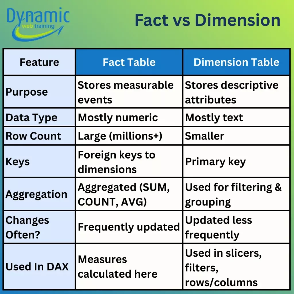
In practice, a model consists of fact tables and dimension tables.
- Fact Tables: Fact tables store events or transactions and contain numeric measures, for example, sale orders table. A fact table is typically very large and grows over time.
- Dimension Tables: Dimension tables describe entities, for example, Products, Customers, Dates with a unique key and a descriptive attribute for filtering, grouping and slicing in reports. They usually have a small number of rows relative to the fact table. Each has a primary key that matches a foreign key in the fact table, plus descriptive attributes such as product name, category, store region or date attributes.
This distinction between fact and dimension tables is a foundational topic in Power BI training courses because nearly every performance issue traces back to modelling mistakes.
A true semantic model always uses fact and dimension tables with one-to-many relationships; the “one” side is the dimension table. Avoid mixing them in a single table. For example, putting product categories, customer names, and sales all in a single “Sales” table not only bloats the table but also makes measure calculations error prone. Keeping tables separated ensures that DAX filter contexts propagate cleanly from dims to facts, and each table’s columns compress efficiently.
Why not use a single flat table?
Sometimes users load all data into one large table instead of separate facts and dimensions. While Power BI will “work” with a single table, this is not a true semantic model. Flattening facts and dimensions into one huge table generally creates a bigger model that only marginally speeds up trivial queries yet performs much worse on real analytical queries.
By contrast, a true semantic model separates facts and dims. Dimension tables enable slicing and filtering, while fact tables enable aggregation. This clean separation is what Power BI’s engine (VertiPaq) is optimized for.
Normalized vs Denormalized Data:
- Normalised data (relational design): Data is split into multiple related tables, so each fact is stored once, reducing redundancy and protecting integrity (often described via normal forms such as 3NF).
- Denormalised data (performance/usage optimisation): Data is intentionally restructured to reduce joins and improve read/query usability by pre-joining commonly accessed attributes. This is done after a sound normalised design exists.
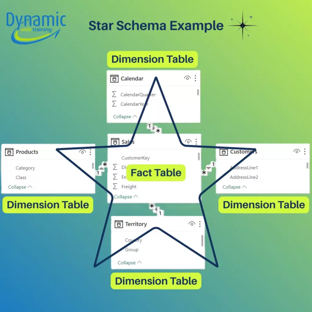
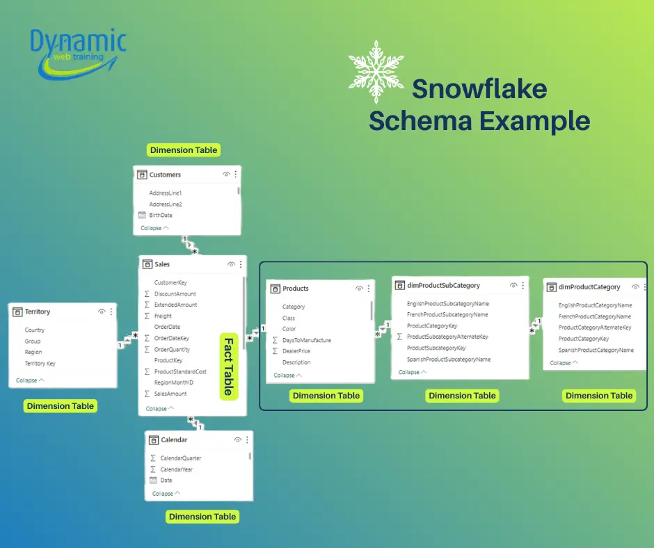
In Power BI we most often use a star schema or a snowflake schema. A star schema has one central fact table and multiple dimension tables radiating out from it. A snowflake schema normalizes one or more dimensions into sub-tables: one or more dimension tables are split into related lookup tables (like Product → ProductCategory → ProductSubcategory).
These schemas have different trade-offs in Power BI:
Star and Snowflake Schemas Defined
- Star Schema: The fact table directly joins to each dimension table. One fact table with simple one-to-many relationships to each dimension. There are no intermediate lookup tables. All descriptive attributes for an entity live in one table. This “flat” dimensional design minimizes joins. This layout resembles a star with the fact at the centre. Star schemas are simple to understand: one dimension equals one table. Star designs also make DAX measures straightforward: filters from slicers flow directly to the fact table through single relationships.
- Snowflake Schema: A variation where one or more dimension tables are normalized. That is, a dimension is split into sub tables. For example, instead of one Product table with Category and Subcategory columns, they have separate Category → Subcategory → Product tables linked in a chain. The structure “branches out” more like a snowflake. Snowflaking reduces data duplication: common attributes like category names live only in one table. However, it adds complexity: each fact-to-dimension filter must traverse multiple tables. For instance, filtering on a product category now requires a join from Fact→Product→Subcategory→Category rather than directly Fact→Product. This eliminates duplicated attributes but creates extra tables.
Comparison: Star vs Snowflake in Power BI
| Aspect | Star Schema | Snowflake Schema |
|---|---|---|
| Query Performance | Fewer joins, faster queries. VertiPaq compresses star-schema tables very efficiently, and repeated dimension values shrink well. Result: visuals and DAX calculations run very quickly. | More joins, slower queries. Snowflake schemas introduce extra relationship “hops” through sub-dimensions, which adds processing overhead. Each additional join can slow down VertiPaq’s in-memory engine. In practice, complex filter propagation through multiple tables degrades performance compared to a star model. |
| DAX Complexity | Simpler. With one dimension table per entity, filter contexts flow cleanly. Functions like CALCULATE or time-intelligence behave predictably. It’s easy to define measures because each filter comes from a single table. | More complex. Filters must traverse intermediate tables, making DAX harder to write and debug. Multi-hop relationships can lead to unexpected filter behavior. For example, you need to explicitly bridge relationships or use CROSSFILTER/USERELATIONSHIP in some cases. |
| Model Size (Memory) | Potentially larger. Dimensions are denormalized, so attribute values are stored redundantly, for example category names repeat for each product row. This can increase model size, but VertiPaq’s columnar compression often offsets the redundancy. | Potentially smaller. Normalization eliminates duplicate attribute storage, e.g. one Category name stored once instead of many times, so raw data size can shrink. However, splitting tables can actually increase overhead per table. In other words, many small tables may not compress as well as a few larger ones. |
| Maintenance and Governance | Simpler to manage. Each dimension is a single table, so updating attributes, adding a column, fixing data, is straightforward. Hierarchies can be defined within one table. Business users and new developers find a star model easier to understand. | More complex. A logical dimension is spread across several tables. Adding a new attribute may mean modifying multiple tables and relationships. Changes in one subtable e.g. adding a new category must be propagated to related tables. |
Real-World Considerations
- Preferred Approach: For almost all Power BI projects, star schema is the starting point. Microsoft and Power BI experts consistently recommend flattening normalized structures when loading data into Power BI.
- VertiPaq Engine: Always remember that Power BI’s VertiPaq stores data column-wise. It loads only the needed columns for each query. Star schemas align perfectly with this: common dimension columns (like category or year) have many repeated values, so they compress extremely well, and since there are fewer relationships, filter contexts are applied quickly. Snowflaked dimensions increase column cardinality and add joins, which means VertiPaq has more work.
Best Practices
- Start with Star Schema: Design your model with one fact table and clear dimension tables wherever possible. This ensures optimal performance and simplicity.
- Use Power Query to Denormalize: If your source has normalized tables, merge them in Power Query to present a star layout to Power BI.
- Monitor Query Plans: Tools like DAX Studio or Power BI’s Performance Analyzer can reveal if extra relationships are costing time. Use these to identify bottlenecks caused by a snowflake design.
- Maintain Clear Documentation: Always document the relationships and reasons. Complex models are harder for colleagues to use correctly.
Conclusion
In summary, Star schemas yield fast queries, simple DAX, and user-friendly models. Snowflake schemas offer space savings and normalized data integrity but require more complex modelling and can slow down visuals. Align your model to your scenario: if speed and simplicity dominate, go star; if data conformity and storage are paramount, consider snowflake. In all cases, follow best practices: drop unused columns, enforce correct data types, and prefer filtering by one-to-many relationships. By doing so, you’ll get the most out of VertiPaq, achieve faster refreshes, and write clearer DAX, whether your model is a star, a snowflake, or a hybrid of both.
If you want to build production-ready data models and truly master dimensional design, consider our advanced Power BI training that goes beyond report building and focuses on modelling fundamentals, performance optimization, and real-world case studies.