
To freeze panes in Excel, go to the View tab and click Freeze Panes in the Window group. Choose Freeze Top Row to keep your headings visible, or Freeze First Column to keep the left column visible. To freeze several rows and columns at once, select the cell immediately below and to the right of the rows and columns you want to lock (for example C3 to lock rows 1 to 2 and columns A to B), then choose Freeze Panes. To undo it, click Freeze Panes > Unfreeze Panes.
When you scroll down a long spreadsheet, the headings disappear and you lose track of which column is which. Freeze Panes fixes that by locking rows or columns in place while the rest of the sheet scrolls. This guide shows you how to freeze the top row, the first column, multiple rows and columns together, how to unfreeze, and what to do when Freeze Panes does not behave.
What does Freeze Panes do in Excel?
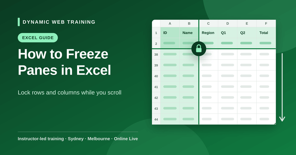
Freeze Panes keeps selected rows at the top, or columns on the left, visible while you scroll through the rest of the worksheet. It changes only what you see on screen; it does not move, protect or change any data. Each worksheet has its own frozen panes, so freezing one sheet does not affect the others.
How do you freeze the top row in Excel?
- Go to the View tab.
- In the Window group, click Freeze Panes.
- Choose Freeze Top Row.
A thin grey line appears under row 1, and the row stays in place as you scroll down. To lock column A instead, choose Freeze First Column from the same menu.
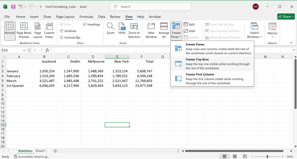
On a Mac, Freeze Panes, Freeze Top Row and Freeze First Column appear on the View tab. In Excel for the web, use View > Freeze Panes.
How do you freeze multiple rows in Excel?
Freeze Top Row only locks row 1. If your headings take up more than one row (for example a title in row 1 and column headings in row 3), freeze them all:
- Select the row directly below the last row you want to freeze. To freeze rows 1 to 3, click the row 4 heading (or cell A4).
- Go to View > Freeze Panes > Freeze Panes.
Everything above the selected row stays visible as you scroll.
How do you freeze columns in Excel?
The same logic works sideways. To freeze columns A and B, select the column C heading (or cell C1), then go to View > Freeze Panes > Freeze Panes. Everything to the left of the selected column stays in place as you scroll right. This is handy for keeping names or ID numbers visible in wide spreadsheets.
How do you freeze rows and columns at the same time?
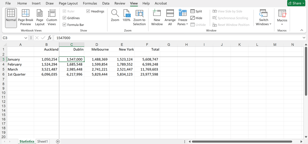
Select the cell that is one row below and one column to the right of the area you want to lock, then choose View > Freeze Panes > Freeze Panes. Excel freezes every row above that cell and every column to its left.
- Select B2 to freeze row 1 and column A.
- Select C3 to freeze rows 1 to 2 and columns A to B.
- Select D5 to freeze rows 1 to 4 and columns A to C.
How do you unfreeze panes in Excel?
Go to View > Freeze Panes and choose Unfreeze Panes. When panes are frozen, this option replaces Freeze Panes at the top of the menu. To change what is frozen, unfreeze first, select a new cell, then freeze again.
Why is Freeze Panes not working?
If Freeze Panes is greyed out or freezes the wrong area, check these:
- You are in Page Layout view. Freeze Panes is not available in Page Layout view. Switch to View > Normal.
- You are editing a cell. Press Enter or Esc to finish editing first.
- The wrong rows are frozen. Excel freezes what is above and to the left of the selected cell as it appears on screen. If you had scrolled down, rows above the window stay hidden. Press Ctrl + Home to go back to the top, then freeze again.
- You can scroll both sections independently. That is Split, not Freeze Panes. Click View > Split to turn it off, then use Freeze Panes.
How do you repeat header rows when printing?
Freeze Panes only affects the screen, not the printout. To print your headings at the top of every page:
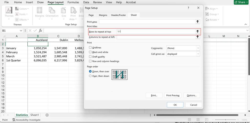
- Go to Page Layout > Print Titles.
- Click in Rows to repeat at top and select your heading rows (for example 1).
- Click OK, then check File > Print to preview.
Practice on your own spreadsheet
Freezing your headings is one of the quickest ways to make a large spreadsheet easier to read and harder to get wrong. Open a long list you work with, freeze the heading row and ID column, and scroll. You will not go back. For more time-savers, see our 30 Excel shortcuts that save hours.
Worksheet navigation, layout and printing are covered in our instructor-led Excel training courses, in-class in Sydney and Melbourne or Online Live across Australia. For the bigger picture, see our Complete Guide to Microsoft Excel.
Frequently asked questions
Go to the View tab, click Freeze Panes in the Window group and choose Freeze Top Row, Freeze First Column or Freeze Panes. For Freeze Panes, first select the cell below and to the right of the rows and columns you want to lock.
Go to View > Freeze Panes > Freeze Top Row. Row 1 stays visible while you scroll down. If your headings are in a lower row, select the row below them and choose Freeze Panes instead.
Select the row directly below the last row you want to keep visible (for example row 4 to freeze rows 1 to 3), then go to View > Freeze Panes > Freeze Panes.
Select the cell one row below and one column to the right of the area you want to lock, such as B2 to freeze row 1 and column A, then go to View > Freeze Panes > Freeze Panes.
Go to View > Freeze Panes and choose Unfreeze Panes. To change the frozen area, unfreeze first, select a new cell and freeze again.
There is no single default shortcut, but you can press the ribbon keys Alt, W, F, F for Freeze Panes (or Unfreeze Panes), Alt, W, F, R for Freeze Top Row, and Alt, W, F, C for Freeze First Column.
